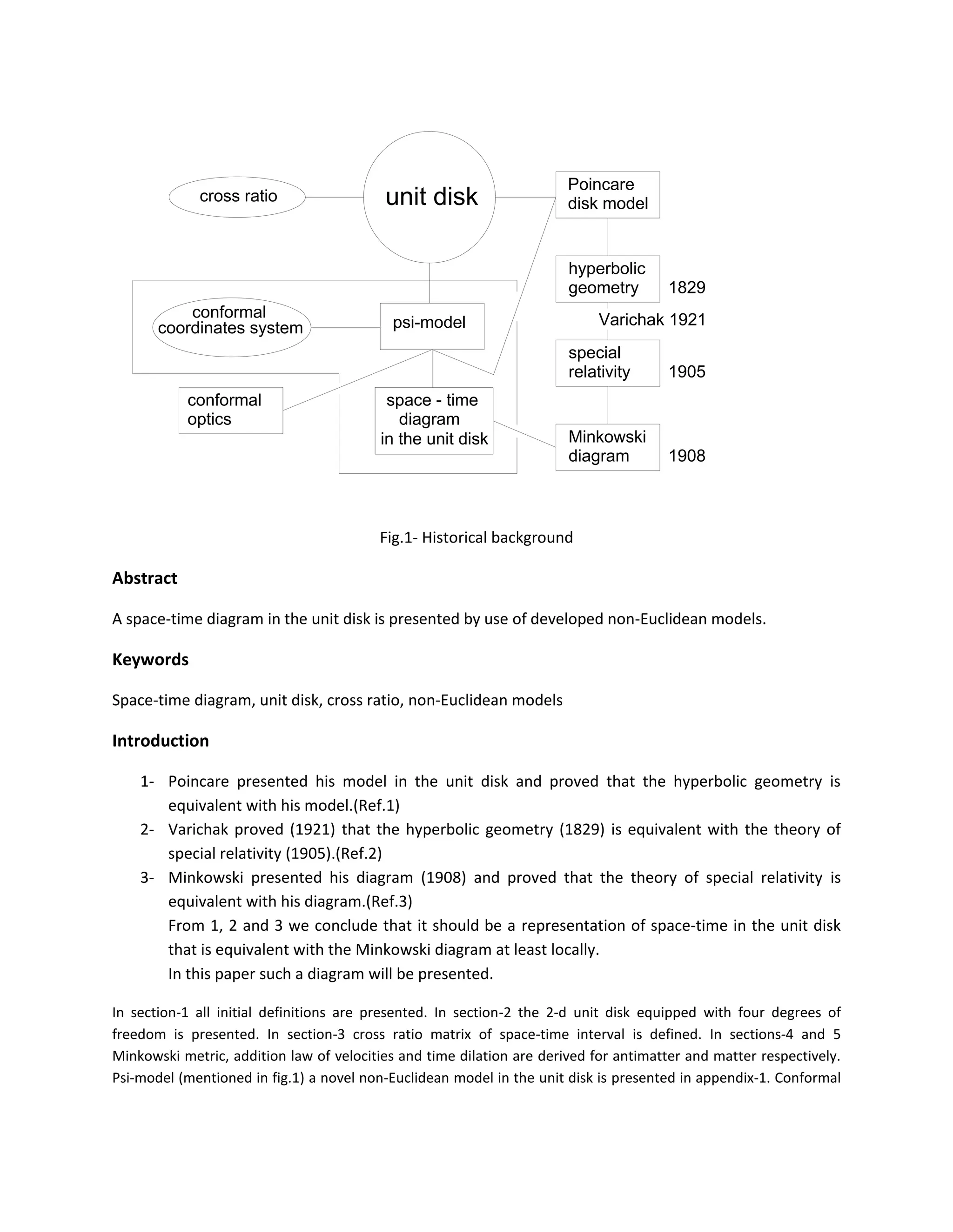
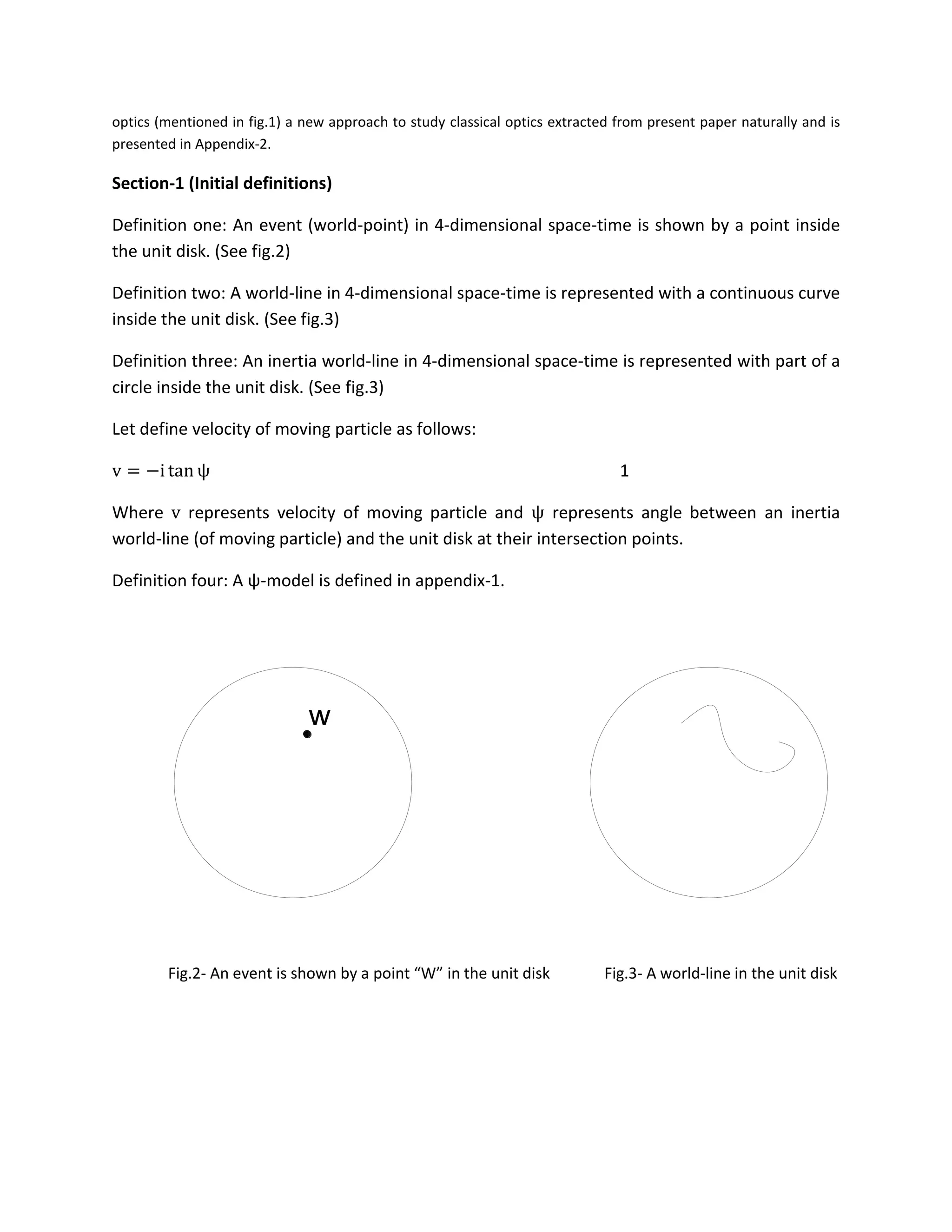
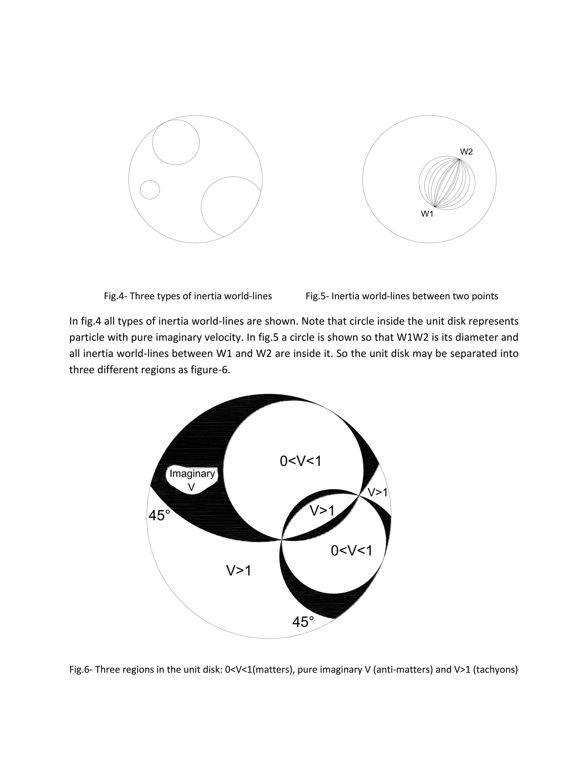
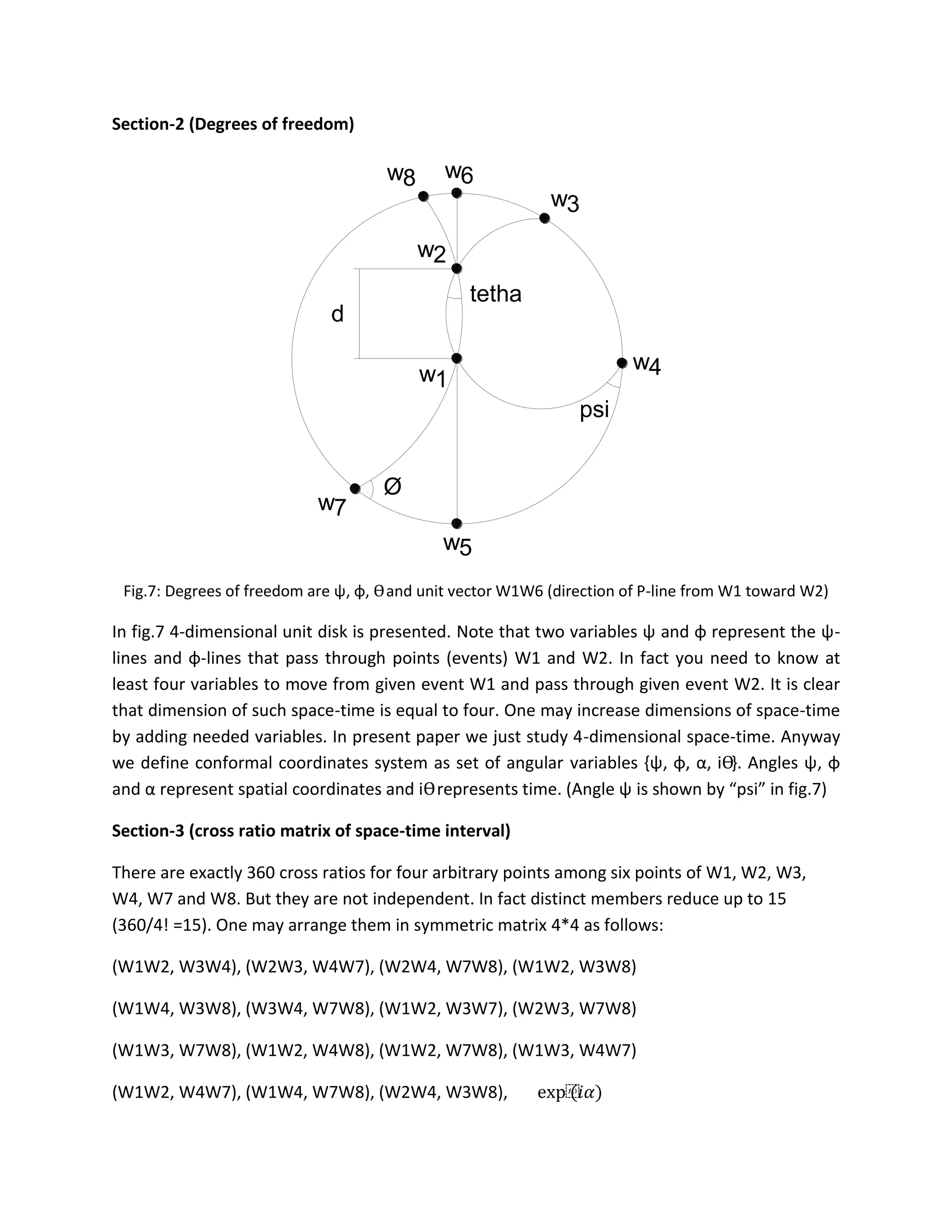
Space-time diagram in the unit disc
From non-Euclidean models to space-time diagram in the unit disk
3/25/2015
cross ratio unit disk
Poincare
disk model
hyperbolic
geometry
special
relativity
Minkowski
diagram
conformal
coordinates system psi-model
space - time
diagram
conformal
optics
in the unit disk
1829
1905
1908
Varichak 1921
Fig.1- Historical background
Abstract
A space-time diagram in the unit disk is presented by use of developed non-Euclidean models.
Keywords
Space-time diagram, unit disk, cross ratio, non-Euclidean models
Introduction
1- Poincare presented his model in the unit disk and proved that the hyperbolic geometry is
equivalent with his model.(Ref.1)
2- Varichak proved (1921) that the hyperbolic geometry (1829) is equivalent with the theory of
special relativity (1905).(Ref.2)
3- Minkowski presented his diagram (1908) and proved that the theory of special relativity is
equivalent with his diagram.(Ref.3)
From 1, 2 and 3 we conclude that it should be a representation of space-time in the unit disk
that is equivalent with the Minkowski diagram at least locally.
In this paper such a diagram will be presented.
In section-1 all initial definitions are presented. In section-2 the 2-d unit disk equipped with four degrees of
freedom is presented. In section-3 cross ratio matrix of space-time interval is defined. In sections-4 and 5
Minkowski metric, addition law of velocities and time dilation are derived for antimatter and matter respectively.
Psi-model (mentioned in fig.1) a novel non-Euclidean model in the unit disk is presented in appendix-1. Conformal
optics (mentioned in fig.1) a new approach to study classical optics extracted from present paper naturally and is
presented in Appendix-2.
Section-1 (Initial definitions)
Definition one: An event (world-point) in 4-dimensional space-time is shown by a point inside
the unit disk. (See fig.2)
Definition two: A world-line in 4-dimensional space-time is represented with a continuous curve
inside the unit disk. (See fig.3)
Definition three: An inertia world-line in 4-dimensional space-time is represented with part of a
circle inside the unit disk. (See fig.3)
Let define velocity of moving particle as follows:
v = −i tan ψ 1
Where v represents velocity of moving particle and ψ represents angle between an inertia
world-line (of moving particle) and the unit disk at their intersection points.
Definition four: A ψ-model is defined in appendix-1.
w
Fig.2- An event is shown by a point “W” in the unit disk Fig.3- A world-line in the unit disk
W2
W1
Fig.4- Three types of inertia world-lines Fig.5- Inertia world-lines between two points
In fig.4 all types of inertia world-lines are shown. Note that circle inside the unit disk represents
particle with pure imaginary velocity. In fig.5 a circle is shown so that W1W2 is its diameter and
all inertia world-lines between W1 and W2 are inside it. So the unit disk may be separated into
three different regions as figure-6.
Imaginary
V>1
V>1
V>1
45°
45°
V
0<V<1
0<V<1
Fig.6- Three regions in the unit disk: 0<V<1(matters), pure imaginary V (anti-matters) and V>1 (tachyons)
Section-2 (Degrees of freedom)
w1
w2
w3
w6
w5
w4
d
w8
w7
Ø
psi
tetha
Fig.7: Degrees of freedom are ψ, φ, ϴand unit vector W1W6 (direction of P-line from W1 toward W2)
In fig.7 4-dimensional unit disk is presented. Note that two variables ψ and φ represent the ψ-
lines and φ-lines that pass through points (events) W1 and W2. In fact you need to know at
least four variables to move from given event W1 and pass through given event W2. It is clear
that dimension of such space-time is equal to four. One may increase dimensions of space-time
by adding needed variables. In present paper we just study 4-dimensional space-time. Anyway
we define conformal coordinates system as set of angular variables {ψ, φ, α, iϴ}. Angles ψ, φ
and α represent spatial coordinates and iϴrepresents time. (Angle ψ is shown by “psi” in fig.7)
Section-3 (cross ratio matrix of space-time interval)
There are exactly 360 cross ratios for four arbitrary points among six points of W1, W2, W3,
W4, W7 and W8. But they are not independent. In fact distinct members reduce up to 15
(360/4! =15). One may arrange them in symmetric matrix 4*4 as follows:
(W1W2, W3W4), (W2W3, W4W7), (W2W4, W7W8), (W1W2, W3W8)
(W1W4, W3W8), (W3W4, W7W8), (W1W2, W3W7), (W2W3, W7W8)
(W1W3, W7W8), (W1W2, W4W8), (W1W2, W7W8), (W1W3, W4W7)
(W1W2, W4W7), (W1W4, W7W8), (W2W4, W3W8), exp⁡(𝑖𝛼)
Where “α” represents direction of Poincare-line from W1 toward W2
Cross ratio matrix Ϯmay be divided in two symmetric matrices as follows:
Amplitude matrix Ϯ𝐴 = 𝐴𝑏𝑠𝑜𝑙𝑢𝑡𝑒 𝑊𝑖 𝑊𝑗 , 𝑊𝑝 𝑊𝑞 = 𝐴𝑏𝑠[
WiWp
W𝑗W𝑝
WjWq
W𝑖W𝑞
] 2
Phase matrix Ϯ𝑃 =
( 𝑊 𝑖 𝑊 𝑗 ,𝑊𝑝 𝑊𝑞 )
𝐴𝑏𝑠𝑜𝑙𝑢𝑡𝑒( 𝑊 𝑖 𝑊 𝑗 ,𝑊𝑝 𝑊𝑞 )
3
Simple calculations yield:
Ϯ𝑃 1,1 = 1 Ϯ𝑃 1,1 = 𝑒 𝑖𝜓
Ϯ𝑃 1,1 = 𝑒 𝑖𝜑
Ϯ𝑃 1,1 = 𝑒 𝑖𝛳
Ϯ𝑃 1,1 = 𝑒 𝑖𝜓
Ϯ𝑃 1,1 = 1 Ϯ𝑃 1,1 = 𝑒 𝑖𝛳
Ϯ𝑃 1,1 = 𝑒 𝑖𝜑
Ϯ𝑃 1,1 = 𝑒 𝑖𝜑
Ϯ𝑃 1,1 = 𝑒 𝑖𝛳
Ϯ𝑃 1,1 = 1 Ϯ𝑃 1,1 = 𝑒 𝑖𝜓
Ϯ𝑃 1,1 = 𝑒 𝑖𝛳
Ϯ𝑃 1,1 = 𝑒 𝑖𝜑
Ϯ𝑃 1,1 = 𝑒 𝑖𝜓
Ϯ𝑃 1,1 = 𝑒 𝑖𝛼
Fig.8: Symmetric 4*4 phase matrix of cross ratio
Calculations of amplitude matrix are more complicated. Referring to fig.7 results are as follows:
Ϯ𝐴 1,1 =
1−𝑡𝑎𝑛 𝜓 𝑡𝑎𝑛 (𝑑 𝑐𝑜𝑠 𝜓)
1+𝑡𝑎𝑛 𝜓 𝑡𝑎𝑛 (𝑑 𝑐𝑜𝑠 𝜓)
4
Ϯ𝐴 3,3 =
1−𝑡𝑎𝑛 𝜑 𝑡𝑎𝑛 (𝑑 𝑐𝑜𝑠 𝜑)
1+𝑡𝑎𝑛 𝜑 𝑡𝑎𝑛 (𝑑 𝑐𝑜𝑠 𝜑)
5
ϮA 4,4 = 1 6
Ϯ𝐴 2,2 = W3W4, W7W8 = (
W3W7
W3W8
)(
W4W8
W4W7
) 7
W3W7 =
2 1 − cos 𝜓 cos 𝜑{ 1 − 𝑑2 (cos 𝜓)2 tan 𝜓 + 𝑑 cos 𝜓 1 − 𝑑2 (cos 𝜑)2 tan 𝜑 + 𝑑 cos 𝜑 + 1 − 𝑑2 (cos 𝜓)2 − 𝑑 sin 𝜓 1 − 𝑑2 (cos 𝜑)2 − 𝑑 sin 𝜑 }
W3W8 =
2 1 − cos 𝜓 cos 𝜑{ 1 − 𝑑2 (cos 𝜓)2 tan 𝜓 + 𝑑 cos 𝜓 1 − 𝑑2 (cos 𝜑)2 tan 𝜑 + 𝑑 cos 𝜑 − 1 − 𝑑2 (cos 𝜓)2 − 𝑑 sin 𝜓 1 − 𝑑2 (cos 𝜑)2 − 𝑑 sin 𝜑 }
lim 𝑑→0 Ϯ𝐴 2,2 = [
cos (
𝜓−𝜑
2
)
cos (
𝜓+𝜑
2
)
]2
8
limd→0 ϮA 1,1 = 1 − 2d sin ψ
tan β
β
, β = d cos ψ 9
W2W3 =
cos (ψ+d cos ψ)
cos ψ
10
W2W4 =
cos (ψ−d cos ψ)
cos ψ
11
W2W7 =
cos (φ−d cos φ)
cos φ
12
W2W8 =
cos (φ+d cos φ)
cos φ
13
ϴ = ϴ1 + ϴ2 , (sin ϴ1/2 = d cos ψ), (sin ϴ2/2 = d cos φ) 14
Section-4 (space interval and time interval)
The most important part of this paper is defining time and spatial intervals correctly. In addition
any model of 4-dimensional space-time in the unit disk must have Minkowski metric locally.
4-1) time interval Δt
Let define time interval Δt between events W1 and W2 as follows:
Δt = iϴ 15
Where ϴ represents intersection angle of ψ-line with φ-line pass through events 𝑊1 and 𝑊2
i = −1
Let assume that variables are time “t” and angle “ψ”. So for small enough “d” we have:
Δt = 2id cos 𝜓 16
Where “d” represents Euclidean distance between W1 and W2 (without any restriction W1 is
located at the center of the unit disk)
And “ψ” represents cut angle between the unit disk and ψ-lines path through W1 and W2.
Note that exactly two ψ-lines path through W1 and W2.
4-2) spatial interval Δσ
Let define spatial interval Δσ between events W1 and W2 as follows:
Δσ = − log[ Ϯ𝐴 1,1 ] = −log⁡(
1−𝑡𝑎𝑛 𝜓 𝑡𝑎𝑛 (d 𝑐𝑜𝑠 𝜓)
1+𝑡𝑎𝑛 𝜓 𝑡𝑎𝑛 (d 𝑐𝑜𝑠 𝜓)
) 17
Note that Poincare metric is derived from equation 17 when ψ=𝛑/2. Anyway for small
enough “d” we have:
Δσ = 2d sin 𝜓 18
4-3) Minkowski metric Δs:
From equations (16) and (18) we have locally:
Δσ2
− Δt2
= 4d2
= (Δ𝑠)2
19
Equation 19 states that Minkowski metric has hold in the unit disk locally.
4-3-1) Velocities adding law
Velocity is defined as follows:
v = Δ𝜎/𝛥𝑡 20
From (16) and (18) we have:
v = −i tan ψ 21
We had defined such velocity before in (1). Now let calculate adding of velocities. Equation (21)
means that
v 𝜓1 + 𝜓2 =
v 𝜓1 +v 𝜓2
1+v 𝜓1 v 𝜓2
22
4-3-2) time dilation
From (16) and (21) we have:
Δt =
Δ𝜏
1−v2
23
Where Δτ represents the proper time
Section-5 (Pure imaginary angle - matters)
Equation (21) states that for real angle of ψ velocity is pure imaginary. Let assume that mass of
“m” has real value. Then kinetic energy of
1
2
mv2
is negative. Negative energy refers to
antimatter. Now let assume that angle of ψ is pure imaginary. Hence velocity of (21) and kinetic
energy of
1
2
mv2
have real values. From (21), (16) and (18) we have:
v = tanh ψ 24
Δt = 2id cosh 𝜓 25
Δσ = 2id sinh 𝜓 26
From (25) and (26) we have:
Δσ2
− Δt2
= 4d2
= (Δ𝑠)2
Also from (24) we have:
v 𝜓1 + 𝜓2 =
v 𝜓1 +v 𝜓2
1+v 𝜓1 v 𝜓2
And finally from (24) and (25) we have:
Δt =
Δ𝜏
1−v2
Section-6 (Conclusion)
It is proved that a representation of space-time in the unit disk exists. Also the space-time
diagram in the unit disk has Minkowski metric locally. The unit disk separated the three regions,
matter region, antimatter region and tachyon region. Since the Minkowski diagram does not
contain the antimatter region, the diagram presented here has more advantages than the
Minkowski one. Space-time interval, addition law of velocities and time dilation equations has
hold for matter and antimatter symmetrically. All results obtained free from customary
coordinates systems. Novel coordinates system applied here called conformal coordinates
system is just in the basis of angles. So all obtained results are invariant under conformal
mappings from physical scene (Appendix-2) to the unit disk.
References
Ref.1 – Poincare disk model, Wikipedia
Ref.2 - Varichak, Wikipedia
Ref.3 – Minkowski diagram, Wikipedia
Appendices
Appendix-1
A non-Euclidean model in the unit disk
Appendix-2
Theory of conformal optics

space-time diagram(final)

  • 1.
    Space-time diagram inthe unit disc From non-Euclidean models to space-time diagram in the unit disk 3/25/2015
  • 2.
    cross ratio unitdisk Poincare disk model hyperbolic geometry special relativity Minkowski diagram conformal coordinates system psi-model space - time diagram conformal optics in the unit disk 1829 1905 1908 Varichak 1921 Fig.1- Historical background Abstract A space-time diagram in the unit disk is presented by use of developed non-Euclidean models. Keywords Space-time diagram, unit disk, cross ratio, non-Euclidean models Introduction 1- Poincare presented his model in the unit disk and proved that the hyperbolic geometry is equivalent with his model.(Ref.1) 2- Varichak proved (1921) that the hyperbolic geometry (1829) is equivalent with the theory of special relativity (1905).(Ref.2) 3- Minkowski presented his diagram (1908) and proved that the theory of special relativity is equivalent with his diagram.(Ref.3) From 1, 2 and 3 we conclude that it should be a representation of space-time in the unit disk that is equivalent with the Minkowski diagram at least locally. In this paper such a diagram will be presented. In section-1 all initial definitions are presented. In section-2 the 2-d unit disk equipped with four degrees of freedom is presented. In section-3 cross ratio matrix of space-time interval is defined. In sections-4 and 5 Minkowski metric, addition law of velocities and time dilation are derived for antimatter and matter respectively. Psi-model (mentioned in fig.1) a novel non-Euclidean model in the unit disk is presented in appendix-1. Conformal
  • 3.
    optics (mentioned infig.1) a new approach to study classical optics extracted from present paper naturally and is presented in Appendix-2. Section-1 (Initial definitions) Definition one: An event (world-point) in 4-dimensional space-time is shown by a point inside the unit disk. (See fig.2) Definition two: A world-line in 4-dimensional space-time is represented with a continuous curve inside the unit disk. (See fig.3) Definition three: An inertia world-line in 4-dimensional space-time is represented with part of a circle inside the unit disk. (See fig.3) Let define velocity of moving particle as follows: v = −i tan ψ 1 Where v represents velocity of moving particle and ψ represents angle between an inertia world-line (of moving particle) and the unit disk at their intersection points. Definition four: A ψ-model is defined in appendix-1. w Fig.2- An event is shown by a point “W” in the unit disk Fig.3- A world-line in the unit disk
  • 4.
    W2 W1 Fig.4- Three typesof inertia world-lines Fig.5- Inertia world-lines between two points In fig.4 all types of inertia world-lines are shown. Note that circle inside the unit disk represents particle with pure imaginary velocity. In fig.5 a circle is shown so that W1W2 is its diameter and all inertia world-lines between W1 and W2 are inside it. So the unit disk may be separated into three different regions as figure-6. Imaginary V>1 V>1 V>1 45° 45° V 0<V<1 0<V<1 Fig.6- Three regions in the unit disk: 0<V<1(matters), pure imaginary V (anti-matters) and V>1 (tachyons)
  • 5.
    Section-2 (Degrees offreedom) w1 w2 w3 w6 w5 w4 d w8 w7 Ø psi tetha Fig.7: Degrees of freedom are ψ, φ, ϴand unit vector W1W6 (direction of P-line from W1 toward W2) In fig.7 4-dimensional unit disk is presented. Note that two variables ψ and φ represent the ψ- lines and φ-lines that pass through points (events) W1 and W2. In fact you need to know at least four variables to move from given event W1 and pass through given event W2. It is clear that dimension of such space-time is equal to four. One may increase dimensions of space-time by adding needed variables. In present paper we just study 4-dimensional space-time. Anyway we define conformal coordinates system as set of angular variables {ψ, φ, α, iϴ}. Angles ψ, φ and α represent spatial coordinates and iϴrepresents time. (Angle ψ is shown by “psi” in fig.7) Section-3 (cross ratio matrix of space-time interval) There are exactly 360 cross ratios for four arbitrary points among six points of W1, W2, W3, W4, W7 and W8. But they are not independent. In fact distinct members reduce up to 15 (360/4! =15). One may arrange them in symmetric matrix 4*4 as follows: (W1W2, W3W4), (W2W3, W4W7), (W2W4, W7W8), (W1W2, W3W8) (W1W4, W3W8), (W3W4, W7W8), (W1W2, W3W7), (W2W3, W7W8) (W1W3, W7W8), (W1W2, W4W8), (W1W2, W7W8), (W1W3, W4W7) (W1W2, W4W7), (W1W4, W7W8), (W2W4, W3W8), exp⁡(𝑖𝛼)
  • 6.
    Where “α” representsdirection of Poincare-line from W1 toward W2 Cross ratio matrix Ϯmay be divided in two symmetric matrices as follows: Amplitude matrix Ϯ𝐴 = 𝐴𝑏𝑠𝑜𝑙𝑢𝑡𝑒 𝑊𝑖 𝑊𝑗 , 𝑊𝑝 𝑊𝑞 = 𝐴𝑏𝑠[ WiWp W𝑗W𝑝 WjWq W𝑖W𝑞 ] 2 Phase matrix Ϯ𝑃 = ( 𝑊 𝑖 𝑊 𝑗 ,𝑊𝑝 𝑊𝑞 ) 𝐴𝑏𝑠𝑜𝑙𝑢𝑡𝑒( 𝑊 𝑖 𝑊 𝑗 ,𝑊𝑝 𝑊𝑞 ) 3 Simple calculations yield: Ϯ𝑃 1,1 = 1 Ϯ𝑃 1,1 = 𝑒 𝑖𝜓 Ϯ𝑃 1,1 = 𝑒 𝑖𝜑 Ϯ𝑃 1,1 = 𝑒 𝑖𝛳 Ϯ𝑃 1,1 = 𝑒 𝑖𝜓 Ϯ𝑃 1,1 = 1 Ϯ𝑃 1,1 = 𝑒 𝑖𝛳 Ϯ𝑃 1,1 = 𝑒 𝑖𝜑 Ϯ𝑃 1,1 = 𝑒 𝑖𝜑 Ϯ𝑃 1,1 = 𝑒 𝑖𝛳 Ϯ𝑃 1,1 = 1 Ϯ𝑃 1,1 = 𝑒 𝑖𝜓 Ϯ𝑃 1,1 = 𝑒 𝑖𝛳 Ϯ𝑃 1,1 = 𝑒 𝑖𝜑 Ϯ𝑃 1,1 = 𝑒 𝑖𝜓 Ϯ𝑃 1,1 = 𝑒 𝑖𝛼 Fig.8: Symmetric 4*4 phase matrix of cross ratio Calculations of amplitude matrix are more complicated. Referring to fig.7 results are as follows: Ϯ𝐴 1,1 = 1−𝑡𝑎𝑛 𝜓 𝑡𝑎𝑛 (𝑑 𝑐𝑜𝑠 𝜓) 1+𝑡𝑎𝑛 𝜓 𝑡𝑎𝑛 (𝑑 𝑐𝑜𝑠 𝜓) 4 Ϯ𝐴 3,3 = 1−𝑡𝑎𝑛 𝜑 𝑡𝑎𝑛 (𝑑 𝑐𝑜𝑠 𝜑) 1+𝑡𝑎𝑛 𝜑 𝑡𝑎𝑛 (𝑑 𝑐𝑜𝑠 𝜑) 5 ϮA 4,4 = 1 6 Ϯ𝐴 2,2 = W3W4, W7W8 = ( W3W7 W3W8 )( W4W8 W4W7 ) 7 W3W7 = 2 1 − cos 𝜓 cos 𝜑{ 1 − 𝑑2 (cos 𝜓)2 tan 𝜓 + 𝑑 cos 𝜓 1 − 𝑑2 (cos 𝜑)2 tan 𝜑 + 𝑑 cos 𝜑 + 1 − 𝑑2 (cos 𝜓)2 − 𝑑 sin 𝜓 1 − 𝑑2 (cos 𝜑)2 − 𝑑 sin 𝜑 } W3W8 = 2 1 − cos 𝜓 cos 𝜑{ 1 − 𝑑2 (cos 𝜓)2 tan 𝜓 + 𝑑 cos 𝜓 1 − 𝑑2 (cos 𝜑)2 tan 𝜑 + 𝑑 cos 𝜑 − 1 − 𝑑2 (cos 𝜓)2 − 𝑑 sin 𝜓 1 − 𝑑2 (cos 𝜑)2 − 𝑑 sin 𝜑 } lim 𝑑→0 Ϯ𝐴 2,2 = [ cos ( 𝜓−𝜑 2 ) cos ( 𝜓+𝜑 2 ) ]2 8 limd→0 ϮA 1,1 = 1 − 2d sin ψ tan β β , β = d cos ψ 9
  • 7.
    W2W3 = cos (ψ+dcos ψ) cos ψ 10 W2W4 = cos (ψ−d cos ψ) cos ψ 11 W2W7 = cos (φ−d cos φ) cos φ 12 W2W8 = cos (φ+d cos φ) cos φ 13 ϴ = ϴ1 + ϴ2 , (sin ϴ1/2 = d cos ψ), (sin ϴ2/2 = d cos φ) 14 Section-4 (space interval and time interval) The most important part of this paper is defining time and spatial intervals correctly. In addition any model of 4-dimensional space-time in the unit disk must have Minkowski metric locally. 4-1) time interval Δt Let define time interval Δt between events W1 and W2 as follows: Δt = iϴ 15 Where ϴ represents intersection angle of ψ-line with φ-line pass through events 𝑊1 and 𝑊2 i = −1 Let assume that variables are time “t” and angle “ψ”. So for small enough “d” we have: Δt = 2id cos 𝜓 16 Where “d” represents Euclidean distance between W1 and W2 (without any restriction W1 is located at the center of the unit disk) And “ψ” represents cut angle between the unit disk and ψ-lines path through W1 and W2. Note that exactly two ψ-lines path through W1 and W2. 4-2) spatial interval Δσ Let define spatial interval Δσ between events W1 and W2 as follows: Δσ = − log[ Ϯ𝐴 1,1 ] = −log⁡( 1−𝑡𝑎𝑛 𝜓 𝑡𝑎𝑛 (d 𝑐𝑜𝑠 𝜓) 1+𝑡𝑎𝑛 𝜓 𝑡𝑎𝑛 (d 𝑐𝑜𝑠 𝜓) ) 17
  • 8.
    Note that Poincaremetric is derived from equation 17 when ψ=𝛑/2. Anyway for small enough “d” we have: Δσ = 2d sin 𝜓 18 4-3) Minkowski metric Δs: From equations (16) and (18) we have locally: Δσ2 − Δt2 = 4d2 = (Δ𝑠)2 19 Equation 19 states that Minkowski metric has hold in the unit disk locally. 4-3-1) Velocities adding law Velocity is defined as follows: v = Δ𝜎/𝛥𝑡 20 From (16) and (18) we have: v = −i tan ψ 21 We had defined such velocity before in (1). Now let calculate adding of velocities. Equation (21) means that v 𝜓1 + 𝜓2 = v 𝜓1 +v 𝜓2 1+v 𝜓1 v 𝜓2 22 4-3-2) time dilation From (16) and (21) we have: Δt = Δ𝜏 1−v2 23 Where Δτ represents the proper time Section-5 (Pure imaginary angle - matters) Equation (21) states that for real angle of ψ velocity is pure imaginary. Let assume that mass of “m” has real value. Then kinetic energy of 1 2 mv2 is negative. Negative energy refers to antimatter. Now let assume that angle of ψ is pure imaginary. Hence velocity of (21) and kinetic energy of 1 2 mv2 have real values. From (21), (16) and (18) we have: v = tanh ψ 24
  • 9.
    Δt = 2idcosh 𝜓 25 Δσ = 2id sinh 𝜓 26 From (25) and (26) we have: Δσ2 − Δt2 = 4d2 = (Δ𝑠)2 Also from (24) we have: v 𝜓1 + 𝜓2 = v 𝜓1 +v 𝜓2 1+v 𝜓1 v 𝜓2 And finally from (24) and (25) we have: Δt = Δ𝜏 1−v2 Section-6 (Conclusion) It is proved that a representation of space-time in the unit disk exists. Also the space-time diagram in the unit disk has Minkowski metric locally. The unit disk separated the three regions, matter region, antimatter region and tachyon region. Since the Minkowski diagram does not contain the antimatter region, the diagram presented here has more advantages than the Minkowski one. Space-time interval, addition law of velocities and time dilation equations has hold for matter and antimatter symmetrically. All results obtained free from customary coordinates systems. Novel coordinates system applied here called conformal coordinates system is just in the basis of angles. So all obtained results are invariant under conformal mappings from physical scene (Appendix-2) to the unit disk. References Ref.1 – Poincare disk model, Wikipedia Ref.2 - Varichak, Wikipedia Ref.3 – Minkowski diagram, Wikipedia Appendices Appendix-1 A non-Euclidean model in the unit disk Appendix-2 Theory of conformal optics