1. Integrales dobles
𝑧 = 𝑓 𝑥, 𝑦 𝐹𝑢𝑛𝑐𝑖ó𝑛 𝑑𝑒 𝑑𝑜𝑠 𝑣𝑎𝑟𝑖𝑎𝑏𝑙𝑒𝑠 𝑑𝑒𝑓𝑖𝑛𝑖𝑑𝑎 𝑒𝑛 𝑢𝑛𝑎 𝑟𝑒𝑔𝑖ó𝑛 𝑅
𝑅 ⊂ ℝ2; Región cerrada
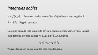
La región cerrada más simple de ℝ2 es la región rectangular cerrada, la cual,
está definida por dos puntos A 𝑎1, 𝑎2 , 𝐵 𝑏1, 𝑏2 , donde
𝑎1 ≤ 𝑏1 𝑦 𝑎2 ≤ 𝑏2
Y cuyos lados son paralelos a los ejes coordenados.
2. La región R se
considerará
como una región
de integración.
R
y
x
4. El primer paso en el estudio de la integral
doble es definir una partición Δ de R
Al dibujar rectas paralelas
a los ejes coordenados se
obtiene una red de
subregiones rectangulares
que cubren a R.
x
y
5. Se tiene n subregiones
• Si tomamos la i-ésima subregión
𝐴𝑛𝑐ℎ𝑜: Δ𝑖𝑥 𝑢𝑛𝑖𝑑𝑎𝑑𝑒𝑠
𝐿𝑎𝑟𝑔𝑜: Δ𝑖𝑦 𝑢𝑛𝑖𝑑𝑎𝑑𝑒𝑠
Ahora, si Δ𝑖𝐴 es el área de la
i-ésima subregión rectangular,
entonces
Δ𝑖𝐴 = Δ𝑖𝑥 ∗ Δ𝑖𝑦
x
y
6. Integral doble
La integral doble proporciona un
valor aproximado del volumen
del sólido que se genera bajo la
función 𝑓 𝑥, 𝑦 definida en una
región R.
Sea 𝑓 𝑥, 𝑦 ≥ 0, y R una región
cerrada, entonces
𝑉 =
𝑅
.
𝑓 𝑥, 𝑦 𝑑𝐴
R
7. Demostración Tenemos una función 𝑓 𝑥, 𝑦 definida
en una región R.
Tomando la i-ésima subregión,
construimos un paralelepípedo sobre
este.
Ahora bien, recordemos que el volumen
del paralelepípedo es igual a
𝑉 = 𝑎𝑛𝑐ℎ𝑜 ∗ 𝑙𝑎𝑟𝑔𝑜 ∗ 𝑎𝑙𝑡𝑢𝑟𝑎
En este caso como estamos trabajando
en la i-ésima subregión, entonces se
tiene que
𝑉𝑖 = Δ𝑖𝑥 ∗ Δ𝑖𝑦 ∗ ℎ𝑖
i-ésima
subregión
?
8. La altura está definida por la función 𝑓.
Si tomamos un punto arbitrario 𝑢𝑖, 𝑣𝑖 de la
i-ésima subregión, entonces
𝑓 𝑢𝑖, 𝑣𝑖 = ℎ𝑖
Por lo tanto,
𝑉𝑖 = Δ𝑖𝑥 ∗ Δ𝑖𝑦 ∗ 𝑓(𝑢𝑖, 𝑣𝑖)
𝑉𝑖 = 𝑓(𝑢𝑖, 𝑣𝑖)Δ𝑖𝑥Δ𝑖𝑦
Pero Δ𝑖𝑥Δ𝑖𝑦 = Δ𝑖𝐴
𝑉𝑖 = 𝑓(𝑢𝑖, 𝑣𝑖)Δ𝑖𝐴
9. 𝑉𝑖 = 𝑓(𝑢𝑖, 𝑣𝑖)Δ𝑖𝐴
𝑉1 = 𝑓(𝑢1, 𝑣1)Δ1𝐴
𝑉2 = 𝑓(𝑢2, 𝑣2)Δ2𝐴
𝑉3 = 𝑓(𝑢3, 𝑣3)Δ3𝐴
…
𝑉𝑖 = 𝑓(𝑢𝑖−1, 𝑣𝑖−1)Δ𝑖𝐴
…
𝑉
𝑛 = 𝑓(𝑢𝑛, 𝑣𝑛)Δ𝑛𝐴
𝑖=1
𝑛
𝑓(𝑢𝑖, 𝑣𝑖)Δ𝑖𝐴
Por lo tanto, el volumen de cada paralelepípedo está dado por
Suma de Riemann
10. Si llevamos al límite esta sumatoria tenemos que
lim
Δ →0
𝑖=1
𝑛
𝑓(𝑢𝑖, 𝑣𝑖)Δ𝑖𝐴
Donde Δ , es la norma de la partición de R y que está determinada por la longitud
de la diagonal más grande de las subregiones rectangulares de la partición.
𝑉 =
𝑅
.
𝑓 𝑥, 𝑦 𝑑𝐴
𝑽 = 𝐥𝐢𝐦
𝜟 →𝟎
𝒊=𝟏
𝒏
𝒇(𝒖𝒊, 𝒗𝒊)𝜟𝒊𝑨
11. • Ejemplo 1: Obtenga un valor aproximado de la integral doble:
𝑅
3𝑦 − 2𝑥2 𝑑𝐴
Donde R es la región rectangular que tiene vértice en (-1,1) y (2,3).
Considere una partición de R generada por las rectas:
x=0, x=1 y y=2,
y tome el centro de la i-ésima subregión como (𝑢𝑖, 𝑣𝑖).
𝑅
3𝑦 − 2𝑥2
𝑑𝐴 ≈
𝑖=1
𝑛
𝑓(𝑢𝑖, 𝑣𝑖)Δ𝑖𝐴
1
𝑥 = 0 𝑥 = 1
y= 2
12. 𝑅
3𝑦 − 2𝑥2
𝑑𝐴 ≈
𝑖=1
𝑛
𝑓(𝑢𝑖, 𝑣𝑖)Δ𝑖𝐴
𝑖=1
𝑛
𝑓(𝑢𝑖, 𝑣𝑖)Δ𝑖𝐴 = 𝑓 𝑢1, 𝑣1 Δ1𝐴 + 𝑓 𝑢2, 𝑣2 Δ2𝐴 + ⋯ + 𝑓 𝑢𝑛, 𝑣𝑛 Δ𝑛𝐴
Para el ejemplo, tenemos que n=6, por lo tanto
𝑖=1
6
𝑓(𝑢𝑖, 𝑣𝑖)Δ𝑖𝐴 = 𝑓 𝑢1, 𝑣1 Δ1𝐴 + 𝑓 𝑢2, 𝑣2 Δ2𝐴 + ⋯ + 𝑓 𝑢6, 𝑣6 Δ6𝐴
ya conocemos los distintos puntos 𝑢𝑖, 𝑣𝑖 (gráfico)
13. Ahora, necesitamos determinar cada Δ𝑖𝐴
Área Δ𝑖𝐴: Como todas la subregiones son iguales, el área de todas estas también van a ser
iguales, es decir,
Δ1𝐴 = Δ2𝐴 = Δ3𝐴 = ⋯ = Δ6𝐴 = 𝐴
y va a estar determinada por
•
•
•
𝐴 = ∆𝑥 ∗ ∆𝑦 𝑑𝑜𝑛𝑑𝑒 Δ𝑥: 𝑎𝑛𝑐ℎ𝑜
Δ𝑦: 𝑙𝑎𝑟𝑔𝑜
𝐴 = 1 ∗ 1
𝐴 = 1
15. Obtenga un valor aproximado de la integral doble:
𝑅
4 −
1
9
𝑥2 −
1
16
𝑦2 𝑑𝐴
Ejercicio propuesto
16. Teoremas:
• 13.2.5: Si c es una constante y la función f es integrable en una región cerrada R,
entonces cf es integrable en R y:
𝑅
𝑐𝑓 𝑥, 𝑦 𝑑𝐴 = 𝑐
𝑅
𝑓 𝑥, 𝑦 𝑑𝐴
• 13.2.6: Si las funciones f y g son integrables en una región cerrada R, entonces la
función f + g es integrable en R y:
𝑅
𝑓 𝑥, 𝑦 + 𝑔 𝑥, 𝑦 𝑑𝐴 =
𝑅
𝑓 𝑥, 𝑦 𝑑𝐴 +
𝑅
𝑔 𝑥, 𝑦 𝑑𝐴
17. • 13.2.7: Si las funciones f y g son integrables en una región cerrada R, y además
f(x,y) ≥ g(x,y) para todo (x,y) de R entonces:
𝑅
𝑓 𝑥, 𝑦 𝑑𝐴 ≥
𝑅
𝑔 𝑥, 𝑦 𝑑𝐴
• 13.2.8: Sea f una función integrable en una región cerrada R, y suponga que m y
M son dos números tales que m ≤ f(x,y) ≤ M para todo (x,y) de R. Si A es la
medida del área del a región R, entonces:
• 13.2.9: Si la función f es continua en la región cerrada R y que la región R se
compone de dos subregiones R1 y R2 que no tienen puntos en común excepto
algunos puntos en parte de sus fronteras. Entonces:
𝑚 ≤
𝑅
𝑓 𝑥, 𝑦 𝑑𝐴 ≤ 𝑀𝐴
𝑅
𝑓 𝑥, 𝑦 𝑑𝐴 =
𝑅1
𝑓 𝑥, 𝑦 𝑑𝐴 +
𝑅2
𝑓 𝑥, 𝑦 𝑑𝐴
19. Integral iterada
Hace referencia a que una integral doble se puede
resolver o determinar mediante integraciones simples
sucesivas.
𝑅
.
𝑓 𝑥, 𝑦 𝑑𝐴 =
𝑎2
𝑏2
𝑎1
𝑏1
𝑓(𝑥, 𝑦) 𝑑𝑥 𝑑𝑦
Integral simple
20. Demostración
𝑉 =
𝑅
.
𝑓 𝑥, 𝑦 𝑑𝐴 =
𝑎2
𝑏2
𝑎1
𝑏1
𝑓(𝑥, 𝑦) 𝑑𝑥𝑑𝑦
Sea z = 𝑓 𝑥, 𝑦 una función definida
en una región R, con 𝑓 𝑥, 𝑦 ≥ 0
21. Recordando un poco acerca de los métodos de integración para
calcular el volumen del sólido generado por una curva, específicamente
el método de rebanadas sabemos que
𝑉 =
𝑎
𝑏
𝐴(𝑦) 𝑑𝑦
Donde A(y), es el área de una sección transversal del sólido.
Para este caso observamos que si integramos con
respecto a 𝑦 el intervalo de integración sería
𝑎, 𝑏 = 𝑎2,𝑏2
Por lo tanto, tendríamos que
𝑉 =
𝑎2,
𝑏2
𝐴(𝑦) 𝑑𝑦
23. Ahora bien, necesitamos determinar 𝐴(𝑦)
Como sabemos 𝐴(𝑦) es la sección transversal de un sólido
𝑨(𝒚)
Nos damos cuenta
que 𝑨(𝒚) está
definida en el
intervalo 𝑎1, 𝑏1
24. Recordando un poco sobre integrales simples, sabemos que la integral definida
determina el área bajo la curva, es decir tenemos que
𝐴 𝑦 =
𝑎1
𝑏1
𝑓(𝑥, 𝑦) 𝑑𝑥
𝑎1 𝑏1
𝒇(𝒙, 𝒚)
A