1. l
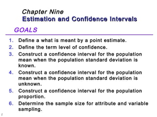
Chapter Nine
Estimation and Confidence IInntteerrvvaallss
GOALS
1. Define a what is meant by a point estimate.
2. Define the term level of confidence.
3. Construct a confidence interval for the population
mean when the population standard deviation is
known.
4. Construct a confidence interval for the population
mean when the population standard deviation is
unknown.
5. Construct a confidence interval for the population
proportion.
6. Determine the sample size for attribute and variable
sampling.

3. Point and Interval Estimates
 A point estimate is a single value (statistic)
used to estimate a population value
(parameter).
 A interval estimate is a range of values within
which the population parameter is expected to
occur.
The interval within which a population
parameter is expected to occur is called a
confidence interval.
The specified probability is called the level of
confidence.
The two confidence intervals that are used
extensively are the 95% and the 99%.

4. Interval Estimation for
The Population Mean
Is the Population Normal
Is n 30 or more ? Is the population standard
deviation known ?
Use a Non
Parametric Test
Use the Z
Distribution
Use the t
Distribution
Use the Z
Distribution
No
No No
Yes
Yes Yes

5. Confidence Intervals
 The degree to which we can rely on the statistic is as
important as the initial calculation. Remember, most
of the time we are working from samples. And
samples are really estimates. Ultimately, we are
concerned with the accuracy of the estimate.
1. Confidence interval provides Range of Values
 Based on Observations from 1 Sample
1. Confidence interval gives Information about
Closeness to Unknown Population Parameter
 Stated in terms of Probability
 Knowing Exact Closeness Requires Knowing
Unknown Population Parameter

6. Areas Under the Normal Curve
Between:
± 1 s - 68.26%
± 2 s - 95.44%
± 3 s - 99.74%
μ
If we draw an observation
from the normal distributed
population, the drawn value is
likely (a chance of 68.26%) to
lie inside the interval of
(μ-1σ, μ+1σ).
P((μ-1σ <x<μ+1σ) =0.6826.
μ-2σ μ+2σ
μ-3σ μ-1σ μ+1σ
μ+3σ

7. Elements of Confidence Interval
Estimation
A probability that the population parameter
falls somewhere within the interval.
Confidence Interval
Sample Statistic
Confidence Limit
(Lower)
Confidence Limit
(Upper)

8. Confidence Intervals
X ±Z×s = ± ×s
X Z n _
m -2.58×s m -1.645×s m m +1.645×s m +2.58×s
m -1.96×s m +1.96×s
90% Samples
95% Samples
99% Samples
sx
X
X
X X X X
X X

9. Level of Confidence
1. Probability that the unknown population
parameter falls within the interval
2. Denoted (1 - a) % = level of confidence
 a Is the Probability That the Parameter Is
Not Within the Interval
1. Typical Values Are 99%, 95%, 90%

10. Interpreting Confidence Intervals
 Once a confidence interval has been
constructed, it will either contain the
population mean or it will not.
 For a 95% confidence interval, if you were to
produce all the possible confidence intervals
using each possible sample mean from the
population, 95% of these intervals would
contain the population mean.

11. Intervals & Level of Confidence
Sampling
Distribution
of Mean
_
a/2 1 - a a/2
Large Number of Intervals
Intervals
Extend from
(1 - a) % of
Intervals
Contain m .
a % Do Not.
m`x = m
X _
sx
- × s
to
X
X Z
X
X Z
+ ×
s

12. Point Estimates and Interval Estimates
X Z s
n
±( a /2)×s = X ±( Z
a /2)×
X
 The factors that determine the width of a
confidence interval are:
1. The size of the sample (n) from which the
statistic is calculated.
2. The variability in the population, usually
estimated by s.
3. The desired level of confidence.

13. Point and Interval Estimates
 If the population standard deviation is known
or the sample is greater than 30 we use the z
distribution.
X ± z s
n

14. CONTOH
 Penelitian dilakukan untuk mengetahui
pendapatan bersih PKL di Surabaya. Dari 100
orang sampel random diketahui rata-rata
pendapatan bersih per hari PKL Rp 50.000
dengan simpangan baku RP 15.000.
Berdasarkan data tersebut lakukan estimasi
pendapatan bersih PKL di Surabaya dengan
tingkat keyakinan 95%.

15. Point and Interval Estimates
 If the population standard deviation is unknown
and the sample is less than 30 we use the t
distribution.
X ±t s
n

16. Student’s t-Distribution
 The t-distribution is a family of distributions
that is bell-shaped and symmetric like the
standard normal distribution but with greater
area in the tails. Each distribution in the t-family
is defined by its degrees of freedom.
As the degrees of freedom increase, the t-distribution
approaches the normal
distribution.

17. About Student
 Student is a pen name for a statistician
named William S. Gosset who was not
allowed to publish under his real name.
Gosset assumed the pseudonym Student for
this purpose. Student’s t distribution is not
meant to reference anything regarding
college students.

18. Zt
Student’s t-Distribution
0
t (df = 5)
Standard
Normal
Bell-Shaped t (df = 13)
Symmetric
‘Fatter’ Tails

19. Upper Tail Area
df .25 .10 .05
1 1.000 3.078 6.314
2 0.817 1.886 2.920
3 0.765 1.638 2.353
0 t
Student’s t Table
Assume:
n = 3
df = n - 1 = 2
a = .10
a/2 =.05
a / 2
t Values 2.920
.05

20. Degrees of freedom
 Degrees of freedom refers to the number of
independent data values available to estimate
the population’s standard deviation. If k
parameters must be estimated before the
population’s standard deviation can be
calculated from a sample of size n, the
degrees of freedom are equal to n - k.

21. Degrees of Freedom (df )
1. Number of Observations that Are Free to Vary After
Sample Statistic Has Been Calculated
2. Example
Sum of 3 Numbers Is 6
X1
= 1 (or Any Number)
X2
= 2 (or Any Number)
X3
= 3 (Cannot Vary)
Sum = 6
degrees of freedom
= n -1
= 3 -1
= 2

22. t-Values
t = x -m
where:
= Sample mean
= Population mean
s = Sample standard deviation
n = Sample size
s
n
xm

23. Estimation Example
Mean (s Unknown)
X
A random sample of n = 25 has = 50 and S = 8.
Set up a 95% confidence interval estimate for m.
X t
S
n
X t
S
- a n - × £ m £ + a n -
×
n - × £ £ + ×
/ , / ,
. .
2 1 2 1
m
m
. £ £
.
50 2 0639
8
25
50 2 0639
8
25
46 69 53 30

24. Central Limit Theorem
 For a population with a mean m and a variance s2
the sampling distribution of the means of all possible
samples of size n generated from the population will
be approximately normally distributed.
 The mean of the sampling distribution equal to m and
the variance equal to s2/n.
The population
X ~ ?(m,s 2 )
distribution
The sample mean of n X ~ N( m , s
2 / n) observation
n

25. Standard Error of the Sample Means
 The standard error of the sample mean is
the standard deviation of the sampling
distribution of the sample means.
 It is computed by
s = s
n x
x s
 is the symbol for the standard error of
the sample mean.
 σ is the standard deviation of the
population.
 n is the size of the sample.

26. Standard Error of the Sample Means
 If s is not known and n ³ 30, the standard
deviation of the sample, designated s , is used
to approximate the population standard
deviation. The formula for the standard error
is:
s s x =
n

27. 95% and 99% Confidence Intervals for
the sample mean
 The 95% and 99% confidence intervals are
constructed as follows:
95% CI for the sample mean is given by
m±1.96 s
n
99% CI for the sample mean is given by
m ±2.58 s
n

28. 95% and 99% Confidence Intervals for μ
 The 95% and 99% confidence intervals are
constructed as follows:
95% CI for the population mean is given by
X ±1.96 s
n
99% CI for the population mean is given by
X ±2.58 s
n

29. Constructing General Confidence
Intervals for μ
 In general, a confidence interval for the mean
is computed by:
X ±z s
n

30. EXAMPLE 3
 The Dean of the Business School wants to
estimate the mean number of hours worked
per week by students. A sample of 49
students showed a mean of 24 hours with a
standard deviation of 4 hours. What is the
population mean?
 The value of the population mean is not
known. Our best estimate of this value is the
sample mean of 24.0 hours. This value is
called a point estimate.

31. Example 3 continued
Find the 95 percent confidence interval for
the population mean.
1.96 24.00 1.96 4
X s
± = ±
24.00 1.12
49
= ±
n
The confidence limits range from 22.88 to
25.12.
About 95 percent of the similarly constructed
intervals include the population parameter.

32. Confidence Interval for a Population
Proportion
 The confidence interval for a population
proportion is estimated by:
p ±z p(1-p)
n

33. EXAMPLE 4
 A sample of 500 executives who own their
own home revealed 175 planned to sell their
homes and retire to Arizona. Develop a 98%
confidence interval for the proportion of
executives that plan to sell and move to
Arizona.
.35 ±2.33 (.35)(.65) = ±
.35 .0497
500

34. CONTOH
 Lembaga riset melakukan penelitian tentang
perusahaan di Jawa Timur yang sudah
menerapkan UMR. Data menunjukkan dari 50
sampel perusahaan, 40 diantaranya sudah
memenuhi UMR. Buatlah confidence interval
90% untuk menduga persentase perusahaan
yang sudah menerapkan UMR.

35. Finite-Population Correction Factor
 A population that has a fixed upper bound is
said to be finite.
 For a finite population, where the total
number of objects is N and the size of the
sample is n , the following adjustment is made
to the standard errors of the sample means
and the proportion:
 Standard error of the sample means:
N n
s s
= -
-1
N
n x

36. Finite-Population Correction Factor
 Standard error of the sample proportions:
N n
p p
= - -
1
(1 )
-
N
n
p s
 This adjustment is called the finite-population
correction factor.
 If n /N < .05, the finite-population correction
factor is ignored.

37. Finite-Population Correction Factor
 Standard error of the sample proportions:
sp
p p
- -
(1 )
n
N n
N
=
-
1
 This adjustment is called the finite-population
correction factor.
 Note : If n/N < 0.05, the finite-population
correction factor is ignored.
 Interval Estimation for proportion with finite-pop
N n
1
ˆ ˆ (1 ˆ )
P p Z p p
= ± - -
-
N
n

38. EXAMPLE 5
 Given the information in EXAMPLE 4,
construct a 95% confidence interval for the
mean number of hours worked per week by
the students if there are only 500 students
on campus.
 Because n /N = 49/500 = .098 which is
greater than 05, we use the finite
population correction factor.
24 1.96( 4 = ±
) 24.00 1.0648
)( 500 49
± -
500 1
49
-

39. CONTOH
 Pimpinan bank ingin mengetahui tentang
kepuasan nasabah terhadap pelayanan bank.
Dari jumlah nasabah 1000 orang, diambil
sampel 100 orang untuk diwawancarai, Hasilnya
60 orang mengakui puas dengan pelayanan
bank tersebut. Dengan a = 5%, berapa proporsi
nasabah yang puas dengan pelayanan bank,

40. Selecting a Sample Size
 There are 3 factors that determine the size
of a sample, none of which has any direct
relationship to the size of the population.
They are:
The degree of confidence selected.
The maximum allowable error.
The variation in the population.

41. Selecting a Sample Size
X Z s
n
±( a /2)×s = X ±( Z
a /2)×
X
 To find the sample size for a variable:
=æ
z * s
÷ø
çè
ö 2 * = E Þ n E
z s
n
where : E is the allowable error, z is the z-
value corresponding to the selected level of
confidence, and s is the sample deviation of the
pilot survey.

42. EXAMPLE 6
 A consumer group would like to estimate the
mean monthly electricity charge for a single
family house in July within $5 using a 99
percent level of confidence. Based on
similar studies the standard deviation is
estimated to be $20.00. How large a sample
is required?
107
(2.58)(20) 2
ö 5
çè
= ÷ø
n = æ

43. Sample Size for Proportions
 The formula for determining the sample size in
the case of a proportion is:
2
n = p - p æ
Z
ö çè
÷ø
( 1 ) E
 where p is the estimated proportion, based on
past experience or a pilot survey; z is the z
value associated with the degree of confidence
selected; E is the maximum allowable error the
researcher will tolerate.

44. EXAMPLE 7
 The American Kennel Club wanted to
estimate the proportion of children that
have a dog as a pet. If the club wanted
the estimate to be within 3% of the
population proportion, how many children
would they need to contact? Assume a
95% level of confidence and that the club
estimated that 30% of the children have a
dog as a pet.
897
(.30)(.70) 1.96
.03
2
= ÷ø
n = æ
ö çè

45. Two-sample Estimation
 Mean :
 n1, n2 ³ 30
m m X X Z s
1 2 1 2 n
 n1, n2 < 30
2
m - m = X - X ± t n - s + n -
s
 Proportion :
ö
æ
( ) ÷ ÷ø
ç çè
2
1
- = - ± +
2
2
2
1
s
n
æ
( ) æ
ö
÷ø
÷ + ÷ ÷ø
ç çè
ö
ç çè
( 1) ( 1)
2 2
1 1
n + n -
n n
2
1 2 1 2
1 2 1 2
1 1
2
ˆ ˆ ˆ (1 ˆ ) ˆ (1 ˆ )
P - P = p - p ± Z p - p + -
( )
p p
2 2
2
1 1
1
1 2 1 2
n
n

46. Contoh
 Perusahaan ban sedang memebandingkan daya
pakai antara ban merek A dan Merek B. Dari
sampel random 10 ban A diketahui rata-rata
daya pakai 1.000 km dengan standar deviasi
100 km sedangkan dari sampel random 10 ban
merek B rata-rata daya pakai 900 km dengan
standar deviasi 90 km. Hitung perbedaan daya
pakai antara ban merek A dan merek B dengan
a = 0,05.

47. Contoh
 Sampel random menunjukkan dari 80 kendaraan
di kota A, 60 diantaranya telah melunasi pajak
sedangkan di kota B dari 70 kendaraan, 40
diantaranya telah melunasi pajak. Hitunglah
perbedaan persentase pelunasan pajak
kendaraan di kedua kota tersebut dengan
tingkat keyakinan 95%.

48. Chapter Nine
Estimation and Confidence IInntteerrvvaallss
- END -