1. The document discusses various algorithms and methods for solving optimization problems involving sparse signal recovery from underdetermined linear systems. 2. Key algorithms mentioned include iterative shrinkage-thresholding algorithms like FISTA, proximal splitting methods like ADMM, and regularization-based methods involving sparse-promoting penalties like l1-norm and sum of absolute values. 3. Applications discussed include compressed sensing, sparse signal recovery from MIMO systems, and discrete signal reconstruction problems.

1. 2019/11/30 @

2. 1.
2.
3.
4.

3. 1.
2.
3.
4.

4. x ∈ ℝN
y = Ax ∈ ℝM
(A ∈ ℝM×N
)
ç
y A x=M = N M N
M < N y A x=M N
̂x = A−1
y
̂x = ✓
✦
✦
x
1/24

5. [1]
✦ MRI [2]
✦ [3]
2/24
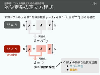
xAy = + v
̂x
x =
0
0
0
1.4
0
0
[1] D. L. Donoho, “Compressed sensing,” IEEE Trans. Inf. Theory, vol. 52, no. 4, pp. 1289–1306, Apr. 2006.
[2] M. Lustig, D. L. Donoho, J. M. Santos, and J. M. Pauly, “Compressed sensing MRI,” IEEE Signal Process. Mag.,
vol. 25, no. 2, pp. 72–82, Mar. 2008.
[3] K. Hayashi, M. Nagahara, and T. Tanaka, “A user’s guide to compressed sensing for communications systems,”
IEICE Trans. Commun., vol. E96-B, no. 3, pp. 685–712, Mar. 2013.

6. ✦ MIMO [4]
✦ [5]
✦ FTN Faster-than-Nyquist [6]
[4] K. K. Wong, A. Paulraj, and R. D. Murch, “Efficient high-performance decoding for overloaded MIMO antenna
systems,” IEEE Trans. Wireless Commun., vol. 6, no. 5, pp. 1833–1843, May 2007.
[5] H. Zhu and G. B. Giannakis, ‘’Exploiting sparse user activity in multiuser detection,’’ IEEE Trans. Commun., vol. 59,
no. 2, pp. 454–465, Feb. 2011.
[6] J. E. Mazo, ‘‘Faster-than-Nyquist signaling,’’ Bell Syst. Tech. J., vol. 54, no. 8, pp. 1451–1462, 1975.
3/24
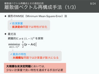
xAy = + v
̂x
x =
1
1
−1
1
−1
−1

7. MIMO
4/24
MIMO (Multiple-Input Multiple-Output)
MIMO
MIMO

8. MIMO
5/24
MIMO
MIMO
✓
-

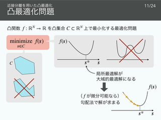
9. MIMO
6/24
˜x1
✦
✦
✦
✦
˜x = [˜x1 ⋯ ˜xNT
] 𝖳
∈ 𝒜NT
˜A =
˜a1,1 ⋯ ˜a1,NT
⋮ ⋱ ⋮
˜aNR,1 ⋯ ˜aNR,NT
∈ ℂNR×NT
˜v = [˜v1 ⋯ ˜vNR
] 𝖳
∈ ℂNR
˜y = [˜y1 ⋯ ˜yNR
] 𝖳
∈ ℂNR
˜xNT
˜a1,1
˜aNR,1
˜a1,NT
˜aNR,NT
˜v1
˜vNR
˜y1
˜yNR
˜y = ˜A˜x + ˜v
QPSK
(Quadrature Phase Shift Keying)
𝒜
Re
Im
𝒜 = {1 + j, − 1 + j,
−1 − j, 1 − j}

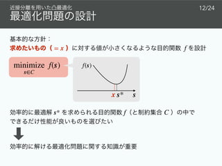
10. MIMO
7/24
MIMO
˜y = ˜A˜x + ˜v ˜x ∈ 𝒜NT
˜y = ˜A˜x + ˜v (˜x ∈ 𝒜NT)
y = Ax + v (x ∈ {1, − 1}2NT)
y =
[
Re{˜y}
Im{˜y}]
∈ ℝ2NR,
(𝒜 = {1 + j, − 1 + j, − 1 − j, 1 − j})
A =
[
Re{ ˜A} −Im{ ˜A}
Im{ ˜A} Re{ ˜A} ]
∈ ℝ2NR×2NT, v =
[
Re{˜v}
Im{˜v}]
∈ ℝ2NR
x =
[
Re{˜x}
Im{˜x}]
∈ {1, − 1}2NT
MIMO =(NR < NT)

11. 1/3
8/24
minimize
s∈{1,−1}N
1
2
∥y − As∥2
2
✦
x ∈ {1, − 1}N
✓
-
✦ MMSE Minimum Mean-Square-Error
✓
-

12. 2/3
9/24
✦
• AMP (Approximate Message Passing) [7]
• EP (Expectation Propagation) [8]
• OAMP (Orthogonal AMP) [9]
• VAMP (Vector AMP) [10]
[7] D. L. Donoho, A. Maleki, and A. Montanari, “Message-passing algorithms for compressed sensing,” Proc. Nat. Acad.
Sci., vol. 106, no. 45, pp. 18914–18919, Nov. 2009.
[8] J. Céspedes, P. M. Olmos, M. Sánchez-Fernández, and F. Perez-Cruz, ‘‘Expectation propagation detection for
high-order high-dimensional MIMO systems,’’ IEEE Trans. Commun., vol. 62, no. 8, pp. 2840–2849, Aug. 2014.
[9] J. Ma and L. Ping, ‘‘Orthogonal AMP,’’ IEEE Access, vol. 5, pp. 2020–2033, 2017.
[10] S. Rangan, P. Schniter, and A. K. Fletcher, ‘’Vector approximate message passing,’’ in Proc. IEEE ISIT, Jun. 2017.
✓
✓
-
-

13. 3/3
10/24
✦
• Box [11]
• regularization-based method [12]
• transform-based method [12]
• SOAV Sum of Absolute Values [13]
[11] P. H. Tan, L. K. Rasmussen, and T. J. Lim, “Constrained maximum-likelihood detection in CDMA,” IEEE Trans.
Commun., vol. 49, no. 1, pp. 142–153, Jan. 2001.
[12] A. Aïssa-El-Bey, D. Pastor, S. M. A. Sbaï, and Y. Fadlallah, “Sparsity-based recovery of finite alphabet solutions to
underdetermined linear systems,” IEEE Trans. Inf. Theory, vol. 61, no. 4, pp. 2008–2018, Apr. 2015.
[13] M. Nagahara, “Discrete signal reconstruction by sum of absolute values,” IEEE Signal Process. Lett., vol. 22, no. 10,
pp. 1575–1579, Oct. 2015.
✓
✓
-

14. 1.
2.
3.
4.

15. f : ℝN
→ ℝ C ⊂ ℝN
minimize
s∈C
f(s) f(s)
s* sC
11/24
f
f(s)
s* s

16. minimize
s∈C
f(s)
= x f
12/24
s* f C
f(s)
s* sx

17. ✦ [16]
✦ FISTA Fast Iterative Shrinkage-Thresholding Algorithm [17]
✦ ADMM Alternating Direction Method of Multipliers [18]
✦ PDS Primal-Dual Splitting [19]
[14] P. L. Combettes and J.-C. Pesquet, “Proximal splitting methods in signal processing,” in Fixed-point algorithms for
inverse problems in science and engineering. Springer, 2011.
[15] , “ ,” ,
vol. 64, no. 6, pp. 316–325, 2019 6 .
[16] P. L. Combettes and V. Wajs, “Signal recovery by proximal forward-backward splitting,” SIAM J. Multi. Model.
Simul., vol. 4, no. 4, pp. 1168–1200, 2005.
[17] A. Beck and M. Teboulle, “A fast iterative shrinkage-thresholding algorithm for linear inverse problems,” SIAM J.
Imag. Sci., vol. 2, no. 1, pp. 183–202, Mar. 2009.
[18] D. Gabay and B. Mercier, “A dual algorithm for the solution of nonlinear variational problems via finite element
approximation,” Comput. Math. Appl., vol. 2, no. 1, pp. 17–40, 1976.
[19] A. Chambolle and T. Pock, “A first-order primal-dual algorithm for convex problems with applications to imaging,”
J. Math. Imaging Vision, vol. 40, no. 1, pp. 120–145, May 2011.
ϕ : ℝN
→ ℝ
proxϕ(s) := arg min
u∈ℝN {
ϕ(u) +
1
2
∥u − s∥2
2}
: ℝN
→ ℝ
13/24

18. FISTA
prox
proxγϕ2
(z) (γ > 0)
+
FISTA
14/24
✓
→
✓ prox [14]
ϕ2(s)
minimize
s∈ℝN
ϕ1(s) + ϕ2(s)
[14] P. L. Combettes and J.-C. Pesquet, “Proximal splitting methods in signal processing,” in Fixed-point algorithms for
inverse problems in science and engineering. Springer, 2011.

19. x ∈ ℝN
y = Ax + v ∈ ℝM
(M < N)
15/24
prox
y − As
∥s∥1 =
N
∑
n=1
|sn|{
✓ =
minimize
s∈ℝN
α
2
∥y − As∥2
2 + ∥s∥1
LASSO (Least Absolute Shrinkage and Selection Operator):

20.
16/24
1.
2. 1.
3. 2. prox
ℓ1

21. 1.
2.
3.
4.

22. ✦
✦
✦
✦
x ∈ {1, − 1}N
A ∈ ℝM×N
(M < N)
v ∈ ℝM
y = Ax + v ∈ ℝM
xAy = + v
̂x
17/24

23. Box [11]
[11] P. H. Tan, L. K. Rasmussen, and T. J. Lim, “Constrained maximum-likelihood detection in CDMA,” IEEE Trans.
Commun., vol. 49, no. 1, pp. 142–153, Jan. 2001.
18/24
Box s ∈ [−1, 1]N
minimize
1−1 s
y − As
s [−1, 1]{
1
2
∥y − As∥2
2
s ∈ [−1, 1]N
x ∈ {1, − 1}N
⊂ [−1, 1]N

24. SOAV [13]
19/24
[13] M. Nagahara, “Discrete signal reconstruction by sum of absolute values,” IEEE Signal Process. Lett., vol. 22, no. 10,
pp. 1575–1579, Oct. 2015.
x ∈ {1, − 1}N
x − 1, x + 1
y − As
∥s − 1∥1, ∥s + 1∥1{
SOAV Sum of Absolute Values
1
2
∥s − 1∥1 +
1
2
∥s + 1∥1 =
N
∑
n=1
(
1
2
|sn − 1| +
1
2
|sn + 1|
)
prox
minimize
s∈ℝN
α
2
∥y − As∥2
2 +
N
∑
n=1
(
1
2
|sn − 1| +
1
2
|sn + 1|
)

25. 1.
2.
3.
4.

26. [20]
20/24
minimize
s∈ℝN
α
2
∥y − As∥2
2 +
1
2
∥s − 1∥1 +
1
2
∥s + 1∥1
SOAV
SSR Sum of Sparse Regularizers
✦
✦
ℓp (0 ≤ p < 1)
ℓ1 − ℓ2
[20] R. Hayakawa and K. Hayashi, ”Discrete-valued vector reconstruction by optimization with sum of sparse
regularizers,” in Proc. EUSIPCO, Sept. 2019.
minimize
s∈ℝN
α
2
∥y − As∥2
2 +
1
2
h(s − 1) +
1
2
h(s + 1)
✓ ADMM PDS

27. [21]
21/24
[21] R. Hayakawa and K. Hayashi, “Reconstruction of complex discrete-valued vector via convex optimization with
sparse regularizers” IEEE Access, vol. 6, pp. 66499–66512, Dec. 2018.
minimize
s∈ℂN
α∥y − As∥2
2 +
L
∑
ℓ=1
qℓhℓ(s − rℓ1)
SCSR Sum of Complex Sparse Regularizers
✦
✦
✦
✦
x ∈ {c1, …, cL}N
⊂ ℂN
A ∈ ℂM×N
(M < N)
v ∈ ℂM
y = Ax + v ∈ ℂM
✓ ADMM
Re
Im
cℓ
Re
Im
cℓ

28. [22] C. Thrampoulidis, E. Abbasi, and B. Hassibi, “Precise error analysis of regularized M-estimators in high dimensions,”
IEEE Trans. Inf. Theory, vol. 64, no. 8, pp. 5592–5628, Aug. 2018.
[23] C. Thrampoulidis, W. Xu, and B. Hassibi, “Symbol error rate performance of box-relaxation decoders in massive
MIMO,” IEEE Trans. Signal Process., vol. 66, no. 13, pp. 3377–3392, Jul. 2018.
22/24
SER
1
N
∥sign( ̂xBox) − x∥0
CGMT Convex Gaussian Min-max Theorem [22, 23]
Box SER Symbol Error Rate
M, N → ∞ (M/N = Δ)
1 − P
(
1
τ* )
SER
Boxx ∈ {1, − 1}N
✦ 0 i.i.d.
✦ 0 i.i.d.
A
v

29. [24] K. Gregor, and Y. LeCun, “Learning fast approximations of sparse coding,” in Proc. ICML, 2010.
[25] S. Takabe, M. Imanishi, T. Wadayama, R. Hayakawa, and K. Hayashi, "Trainable projected gradient detector for
massive overloaded MIMO channels: Data-driven tuning approach,” IEEE Access, vol. 7, pp. 93326-93338, Jul.
2019.
23/24
✦ [24]
MIMO [25]
A
B
C
A B C A B C

30. ✦
✦
✦
24/24