Design of the bell nozzle contour by characteristic method.

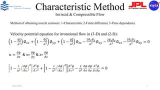
1. Characteristic Method
Inviscid & Compressible Flow
Method of obtaining nozzle contours: 1-Characteristic 2-Finite difference 3-Time dependence
Velocity potential equation for irrotational flow in (3-D) and (2-D):
1 −
1
𝑎2
𝜕𝜙
𝜕𝑥
2 𝜕2𝜙
𝜕𝑥2 + 1 −
1
𝑎2
𝜕𝜙
𝜕𝑦
2 𝜕2𝜙
𝜕𝑦2 −
2
𝑎2
𝜕𝜙
𝜕𝑥
𝜕𝜙
𝜕𝑦
𝜕2𝜙
𝜕𝑥𝜕𝑦
= 0
10/11/2021 1
1 −
∅𝑥
2
𝑎2 ∅𝑥𝑥 + 1 −
∅𝑦
2
𝑎2 ∅𝑦𝑦 + 1 −
∅𝑧
2
𝑎2 ∅𝑧𝑧 −
2∅𝑥∅𝑦
𝑎2 ∅𝑥𝑦 −
2∅𝑥∅𝑧
𝑎2 ∅𝑥𝑧 −
2∅𝑧∅𝑦
𝑎2 ∅𝑧𝑦 = 0
𝑢 =
𝜕𝜙
𝜕𝑥
& v=
𝜕𝜙
𝜕𝑦
& z=
𝜕𝜙
𝜕𝑧

2. 𝜕𝜙
𝜕𝑥
= 𝑢,
𝜕𝜙
𝜕𝑦
=v
10/11/2021 2
1 −
𝑢2
𝑎2
𝜕𝑢
𝜕𝑥
+ 1 −
𝑣2
𝑎2
𝜕𝑣
𝜕𝑦
−
2𝑢𝑣
𝑎2
𝜕𝑢
𝜕𝑦
= 0
𝜕𝜙
𝜕𝑥
= 𝑓(𝑥, 𝑦)
𝑑𝑓 =
𝜕𝑓
𝜕𝑥
ⅆx +
𝜕𝑓
𝜕𝑦
ⅆ𝑦
𝑑
𝜕𝜙
𝜕𝑥
= 𝑑𝑢 =
𝜕2
𝜙
𝜕𝑥2
ⅆx +
𝜕2
𝜙
𝜕𝑥𝜕𝑦
ⅆ𝑦
𝑑
𝜕𝜙
𝜕𝑦
= 𝑑𝑢 =
𝜕2
𝜙
𝜕𝑥𝜕𝑦
ⅆx +
𝜕2
𝜙
𝜕𝑦2
ⅆy
𝜕𝜙
𝜕𝑦
= 𝑓(𝑥, 𝑦)

3. • Therefore for 2-D:
𝜕𝑢
𝜕𝑥 𝑖,𝑗
=
2𝑢𝑣
𝑎2
𝜕𝑢
𝜕𝑦
− (1 −
𝑣2
𝑎2)
𝜕𝑣
𝜕𝑦
1 −
𝑢2
𝑎2
Velocity of the fluid in the flow field:
10/11/2021 3

4. • Writing Taylor series for D:
𝑢𝑖+1,𝑗 = 𝑢𝑖,𝑗 +
𝜕𝑢
𝜕𝑥 𝑖,𝑗
Δ𝑥 +
1
2
𝜕2
𝑢
𝜕𝑥2
(Δ𝑥)2+ ⋯
By ignoring higher orders,
𝜕𝑢
𝜕𝑥 𝑖,𝑗
will be obtain.
The determinator should not be equal to zero to the fraction is to be determinable.
In Mach line definition axial velocity is sonic and then:
1 −
𝑢2
𝑎2=0 so u=a=sonic
10/11/2021 4

5. •
u=a
v
𝑉
𝜇
𝜇
Therefore sin 𝜇 =
𝑎
𝑣
=
1
𝑀
so this is a Mach line meaning
So Mach line is characteristic line
10/11/2021 5

6. 1 −
𝑢2
𝑎2
𝜙𝑥𝑥 −
2𝑢𝑣
𝑎2
𝜙𝑥𝑦 + 1 −
𝑣2
𝑎2
𝜙𝑦𝑦 = 0
• 𝑑𝑥𝜙𝑥𝑥 + 𝑑𝑦 𝜙𝑥𝑦 = 𝑑𝑢 solve for 𝜙𝑥𝑦
• 𝑑𝑥 𝜙𝑥𝑦 + 𝑑𝑦𝜙𝑦𝑦 = 𝑑𝑣
𝜕2𝜙
𝜕𝑥𝜕𝑦
=
1 −
𝑢2
𝑎2 0 1 −
𝑣2
𝑎2
𝑑𝑥 𝑑𝑢 0
0 𝑑𝑣 𝑑𝑦
1 −
𝑢2
𝑎2 −
2𝑢𝑣
𝑎2 1 −
𝑣2
𝑎2
𝑑𝑥 𝑑𝑦 0
0 𝑑𝑥 𝑑𝑦
=
𝑁
𝐷
10/11/2021 6

7. • This fraction will become indeterminate when D=0.
• To have an Char-Line, 𝜙𝑥𝑦 had to be indeterminate.
• For given incremental changes, that the denominator goes to zero then 𝜙𝑥𝑦=
discontinuous.
• If D=0,so:
𝑑𝑦
𝑑𝑥
=
−
𝑢𝑣
𝑎2±(
𝑢2+𝑣2
𝑎2 −1)
1−
𝑢2
𝑎2
: Char-Line eq have to be solved
* 𝑢2 + 𝑣2=𝑉2so
𝑢2+𝑣2
𝑎2 =
𝑉2
𝑎2 = 𝑀2 then
𝑑𝑦
𝑑𝑥
=
−
𝑢𝑣
𝑎2±( 𝑀2−1)
1−
𝑢2
𝑎2
10/11/2021 7

8. 𝐶+
𝐶−
𝑉
𝜇
𝜇
𝜃
Stream line
A
• 𝑢 = 𝑉 cos 𝜃 & 𝑣 = 𝑉 sin 𝜃
By substituting and simplifying,
𝑑𝑦
𝑑𝑥
can be rewritten as:
•
𝑑𝑦
𝑑𝑥
= tan(𝜃 ∓ 𝜇) (char-line Eq)
D tells us how char-lines are located,
what is their orientation and local velocity,
but N does essentially tell us the
relationship of the properties and how they change over the char-line.
10/11/2021 8

9. • We have 3 conditions:
1. M>1: two real roots, two char-line which means super sonic flow, we got
hyperbolic (PDE).
2. M=1: one real root, one char-line/ Sonic case/ Parabolic PDE.
3. M<1: Imaginary roots/ elliptic PDE.
If N=0: To 𝜙𝑥𝑦 =𝑑u/𝑑y = 𝑑𝑣/𝑑x be finite. Since 0<𝑑u/𝑑x<C
𝑑𝑣
𝑑𝑢
= ∓ 𝑀2−1
𝑑𝑣
𝑣
Which is exactly means P-M expansion angle, i.e.,
𝑑𝑣
𝑑𝑢
= ∓ 𝑀2−1 𝑑𝑣
𝑣
= 𝑑𝜃: this is compatibility EQ
10/11/2021 9

10. • According to compatibility Eq and based on char-line Eq:
𝑑𝜃 = − 𝑀2−1
𝑑𝑣
𝑣
: 𝐶−
: 𝑅𝑅𝑤
𝑑𝜃 = + 𝑀2−1
𝑑𝑣
𝑣
: 𝐶+: 𝐿𝑅𝑤
By integrating:
𝐶−
≡ 𝜃 + 𝛾 𝑀 = Constant=𝐾−
𝐶+
≡ 𝜃 − 𝛾 𝑀 = Constant=𝐾+
Where K is a constant parameter along each char-line.
10/11/2021 10

11. • P-M expansion wave angle:
𝜃 = 𝛾 𝑀2 − 𝛾 𝑀1
Where 𝛾 is a P-M function:
𝛾(M)=
𝛾+1
𝛾−1
tan−1 𝛾−1
𝛾+1
(𝑀2 − 1) − tan−1 𝑀2 − 1
𝜃 =
1
2
(𝐾−+ 𝐾+) & 𝛾 =
1
2
(𝐾− − 𝐾+)
10/11/2021 11

12. • Nozzle definition types according to char-line:
Gradually expansion nozzle
Minimum length nozzle
10/11/2021 12

13. 10/11/2021 13

14. P
A
B
• Consider the intersection of two characteristic lines A and B at point P, then we
have:
𝑚1 = tan(
𝜃 − 𝑎 𝐴 + 𝜃 − 𝑎 𝑃
2
)
𝑚11 = tan(
𝜃 − 𝑎 𝐵 + 𝜃 − 𝑎 𝑃
2
)
And
𝑦𝑃 = 𝑦𝐴 + 𝑚1(𝑥𝑃 − 𝑥𝐴)
𝑦𝑃 = 𝑦𝐵 + 𝑚11(𝑥𝑃 − 𝑥𝐵)
𝑥𝑃 =
𝑦1 − 𝑦𝐵 + 𝑚11𝑥𝐵 − 𝑚1𝑥𝐴
𝑚11 − 𝑚1
10/11/2021 14

15. • Inviscid Mach contour
• Diverging length at Mach 3
• RS-25 contour is on MATLAB
(press Ctrl + Clink on it)
Also Solidworks part is here
10/11/2021 15

16. 10/11/2021 16

17. 10/11/2021 17

18. • 𝑝𝑟𝑒𝑠𝑠𝑢𝑟𝑒 𝑟𝑎𝑡𝑖𝑜:
𝑜𝑢𝑡𝑠𝑖𝑑𝑒 𝑝𝑟𝑒𝑠𝑠𝑢𝑟𝑒
𝑐ℎ𝑎𝑚𝑏𝑒𝑟 𝑝𝑟𝑒𝑠𝑠𝑢𝑟𝑒
𝑇𝑒𝑚𝑝 𝑟𝑎𝑡𝑖𝑜: (𝑝𝑟𝑒𝑠𝑠𝑢𝑟𝑒 𝑟𝑎𝑡𝑖𝑜)
𝛾−1
𝛾
• 𝐶𝑟𝑖𝑡𝑖𝑐𝑎𝑙 𝑡ℎ𝑟𝑜𝑎𝑡 𝑇𝑒𝑚𝑝 =
2𝛾𝑅.𝑐ℎ𝑎𝑚𝑏𝑒𝑟 𝑇𝑒𝑚𝑝
𝛾−1
𝐶ℎ𝑒𝑟𝑖𝑡𝑖𝑐𝑎𝑙 𝑡ℎ𝑟𝑜𝑎𝑡 𝑝𝑟𝑒𝑠𝑠𝑢𝑟𝑒 =
2
𝛾+1
𝛾
𝛾−1
∗ 2.088
• 𝐶ℎ𝑒𝑟𝑖𝑡𝑖𝑐𝑎𝑙 𝑡ℎ𝑟𝑜𝑎𝑡 𝑣𝑒𝑙𝑜𝑐𝑖𝑡𝑦 =
2𝛾𝑅.𝐶ℎ𝑎𝑚𝑏𝑒𝑟 𝑇𝑒𝑚𝑝
𝛾+1
• 𝐸𝑥𝑖𝑡 𝑣𝑒𝑙𝑜𝑐𝑖𝑡𝑦 = 𝑇ℎ𝑟𝑜𝑎𝑡 𝑇𝑒𝑚𝑝. (1 − 𝑇𝑒𝑚𝑝 𝑟𝑎𝑡𝑖𝑜)
• 𝐸𝑥𝑖𝑡 𝑇𝑒𝑚𝑝 = 𝐶ℎ𝑎𝑚𝑏𝑒𝑟 𝑇𝑒𝑚𝑝 . (
𝑃𝑒𝑥𝑖𝑡
𝑃𝑐ℎ𝑎𝑚𝑏𝑒𝑟
)
𝛾−1
𝛾
• 𝐸𝑥𝑖𝑡 𝑠𝑜𝑢𝑛𝑑 𝑠𝑝𝑒𝑒𝑑 = 𝛾𝑅𝑇𝑒𝑥𝑖𝑡
• 𝐸𝑥𝑖𝑡 𝑀𝑎𝑐ℎ =
𝑒𝑥𝑖𝑡 𝑣𝑒𝑙𝑜𝑐𝑖𝑡𝑦
𝑒𝑥𝑖𝑡 𝑠𝑜𝑢𝑛𝑑 𝑠𝑝𝑒𝑒𝑑
• 𝑃𝑀 =
𝛾+1
𝛾−1
× tan−1 𝛾−1
𝛾+1
𝑀2 − 1 − tan−1 𝑀2 − 1
• 𝑀𝑎𝑥𝑖𝑚𝑢𝑚 𝑤𝑎𝑙𝑙 𝑎𝑛𝑔𝑙𝑒 =
1
2
{𝑃𝑀(𝑒𝑥𝑖𝑡 𝑀𝑎𝑐ℎ)}
• 𝐴𝑛𝑔𝑙𝑒 𝑖𝑛𝑐𝑟𝑒𝑚𝑒𝑛𝑡 = 2. ( 90 − 𝑀𝑎𝑥 𝑎𝑛𝑔𝑙𝑒 − 𝑓𝑖𝑥 90 − 𝑀𝑎𝑥 𝑎𝑛𝑔𝑙𝑒 )
10/11/2021 18

19. • MATLAB Coding Method:
10/11/2021 19
Exit pressure
Pressure ratio
Throat T,P,V
Exit V,T,a,M
Prandtl-Mayer
function to finding
expansion angle-its
recursive
Maximum Wall
angle
Number of division
Calculate position of
the center line
Calculate the wall
positions- its
recursive
Export X,Y into CAD

20. For more information read Rocket Science book
which is written by Mahdi Hossein gholi nejad
and Professor Mofid Gorji.
With special thanks from
10/11/2021 20