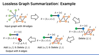
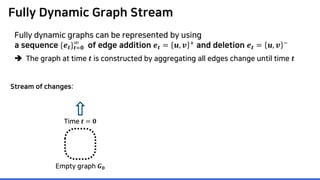
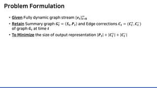
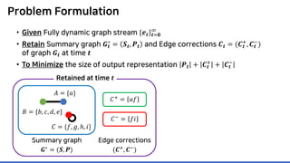
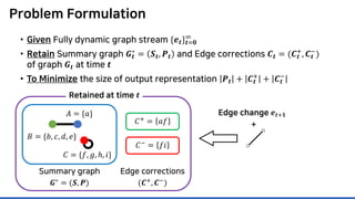
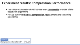
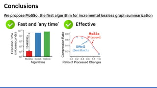
The document discusses incremental lossless graph summarization, highlighting its importance for efficiently manipulating large-scale evolving graphs. It presents a proposed algorithm named Mosso, which updates compressed graphs quickly without needing to rerun algorithms from scratch due to changes in the graph structure. The approach includes the creation of a summary graph and edge corrections to minimize edge count, offering benefits for querying and further compression.


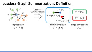
![Lossless Graph Summarization: Definition
Lossless
Summarization
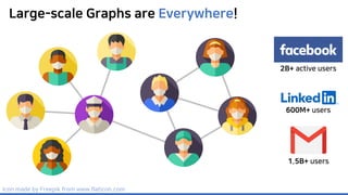
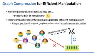
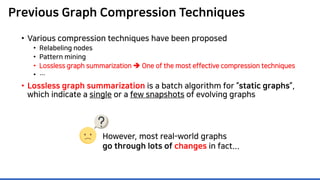
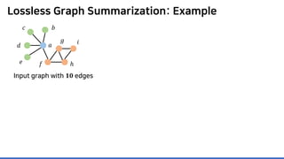
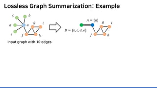
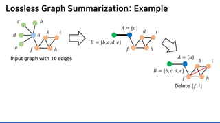
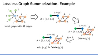
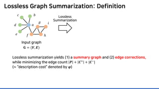
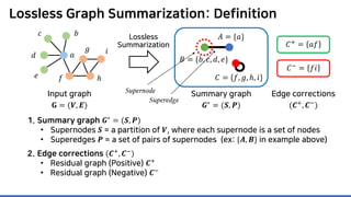
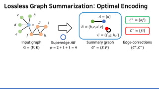
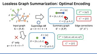
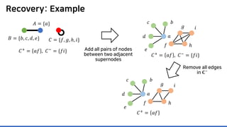
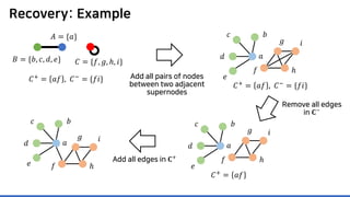
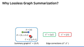
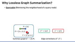
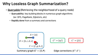
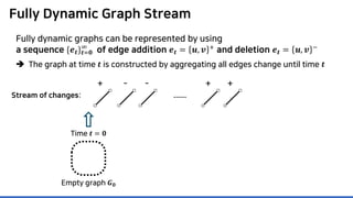
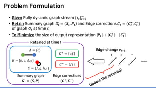
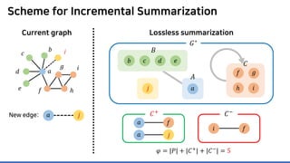
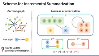
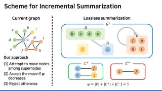
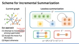
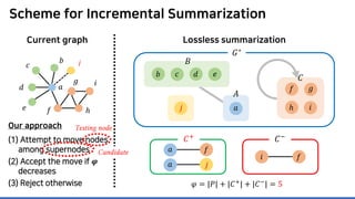
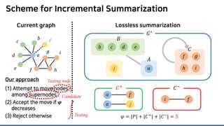
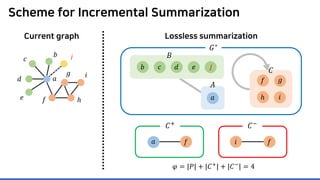
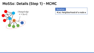
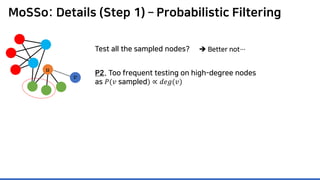
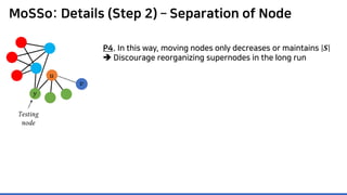
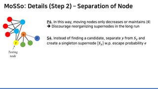
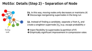
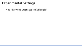
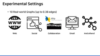
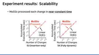
Lossless summarization yields (1) a summary graph and (2) edge corrections,
while minimizing the edge count 𝑷𝑷 + 𝑪𝑪+
+ |𝑪𝑪−
|
(≈ “description cost” denoted by 𝝋𝝋)
Proposed in [NRS08]
based on “the Minimum
Description Length principle”
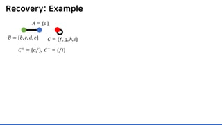
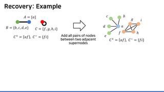
𝐶𝐶+ = 𝑎𝑎𝑎𝑎
𝐶𝐶−
= 𝑓𝑓𝑖𝑖
Summary graph
𝑮𝑮∗ = (𝑺𝑺, 𝑷𝑷)
Edge corrections
(𝑪𝑪+, 𝑪𝑪−)
Input graph
𝐆𝐆 = (𝑽𝑽, 𝑬𝑬)
𝑎𝑎
𝑏𝑏𝑐𝑐
𝑑𝑑
𝑒𝑒 𝑓𝑓
𝑔𝑔
ℎ
𝑖𝑖
𝐴𝐴 = {𝑎𝑎}
𝐵𝐵 = {𝑏𝑏, 𝑐𝑐, 𝑑𝑑, 𝑒𝑒}
𝐶𝐶 = {𝑓𝑓, 𝑔𝑔, ℎ, 𝑖𝑖}](https://image.slidesharecdn.com/presentationvideomossoshare-200823101311/85/Incremental-Lossless-Graph-Summarization-KDD-2020-23-320.jpg)
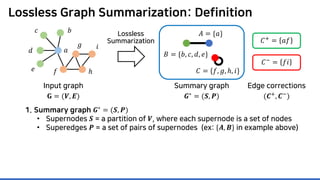
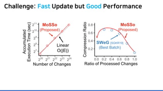
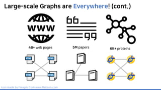
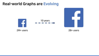
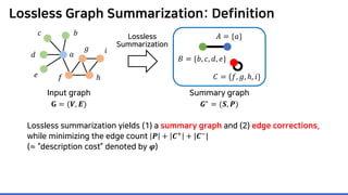
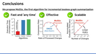
![MoSSo: Details (Step 1) – MCMC
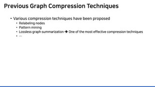
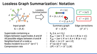
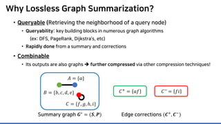
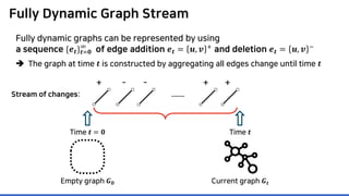
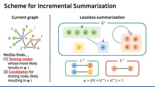
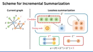
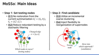
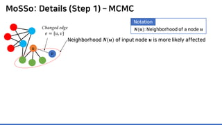
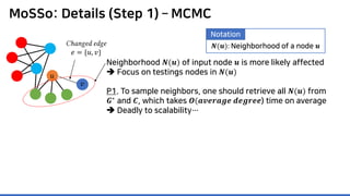
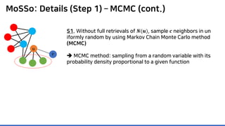
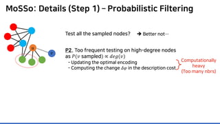
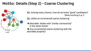
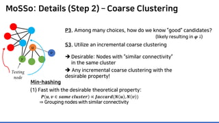
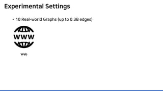
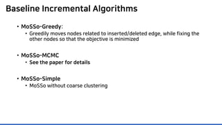
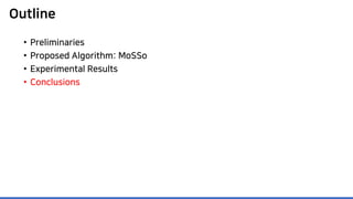
Neighborhood 𝑵𝑵(𝒖𝒖) of input node 𝒖𝒖 is more likely affected
Focus on testings nodes in 𝑵𝑵(𝒖𝒖)
P1. To sample neighbors, one should retrieve all 𝑵𝑵(𝒖𝒖) from
𝑮𝑮∗
and 𝑪𝑪, which takes 𝑶𝑶(𝒂𝒂𝒂𝒂𝒂𝒂𝒂𝒂𝒂𝒂𝒂𝒂𝒂𝒂 𝒅𝒅𝒅𝒅𝒅𝒅𝒅𝒅𝒅𝒅𝒅𝒅) time on average
Deadly to scalability…
𝑢𝑢
𝑣𝑣
Changed edge
𝑒𝑒 = {𝑢𝑢, 𝑣𝑣}
Graph densification law [LKF05]:
“The average degree of real-world graphs increases over time.”
𝑵𝑵(𝒖𝒖): Neighborhood of a node 𝒖𝒖
Notation](https://image.slidesharecdn.com/presentationvideomossoshare-200823101311/85/Incremental-Lossless-Graph-Summarization-KDD-2020-73-320.jpg)


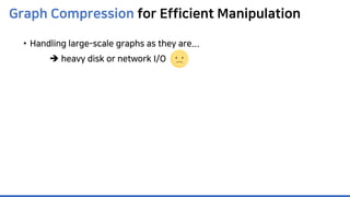
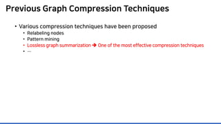
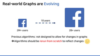
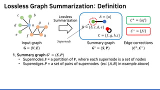
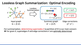
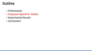
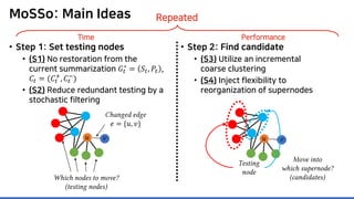
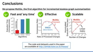
![Experimental Settings
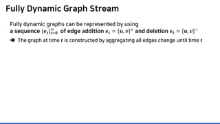
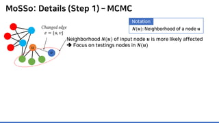
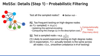
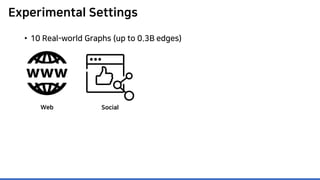
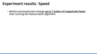
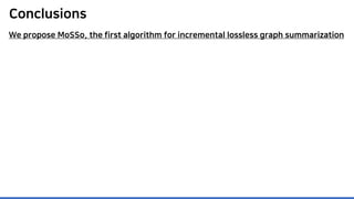
• 10 Real-world Graphs (up to 0.3B edges)
• Batch loseless graph summarization algorithms:
• Randomized [NSR08], SAGS [KNL15], SWeG [SGKR19]
Web Social Collaboration Email And others!](https://image.slidesharecdn.com/presentationvideomossoshare-200823101311/85/Incremental-Lossless-Graph-Summarization-KDD-2020-97-320.jpg)


![Trial pahang 2014 spm add math k2 dan skema [scan]](https://cdn.slidesharecdn.com/ss_thumbnails/trialpahang2014spmaddmathk2danskemascan-141015101353-conversion-gate01-thumbnail.jpg?width=640&height=640&fit=bounds)