3. PREFACE
This volume is the third within the series of textbooks written by Z.E.Heinemann. The
previous volumes:
• Flow in Porous Media
• Reservoir Fluids
deal with the properties of porous media, the one and two phase flow in reservoir rocks,
phase behavior and thermodynamical properties of oil, gas and brine.
To use this volume it is supposed that the reader has attended the courses mentioned above
or possesses profound knowledge of these topics. All methods discussed in this volume
have practical importance and are used in today work. However, it is not possible to give
a complete overview about the whole range of the classical and modern reservoir
engineering tools. The selection was made under the aspect of transmitting basic
understandings about the reservoir processes, rather to provide recipes.
This volume is followed by the textbooks
• Well Testing
• Basic Reservoir Simulation
• Enhanced Oil Recovery
• Advanced Reservoir Simulation Management
The seven volumes cover the whole area of reservoir engineering normally offered in
graduate university programs worldwide, and is specially used at the MMM University
Leoben.
9. I
Table of Contents
Introduction 3
1.1 General Remarks ...................................................................................................................3
1.2 Classification of Reserves .....................................................................................................7
Reserves Calculation by Volumetric Methods 9
2.1 Computation of Oil and Gas in Place ....................................................................................9
2.2 Recovery Factor ..................................................................................................................10
2.3 Data Distribution and Probability .......................................................................................11
2.3.1 Triangular Distribution .........................................................................................14
2.3.2 Uniform Distribution ............................................................................................15
2.3.3 Dependent Distribution .........................................................................................16
2.4 Monte Carlo Simulation Method ........................................................................................17
Material Balance 25
3.1 Tarner’s Formulation ..........................................................................................................25
3.2 Drive Indices .......................................................................................................................29
3.3 Water Influx ........................................................................................................................30
3.3.1 Semi-Steady-State Water Influx ...........................................................................32
3.3.2 Steady-State Water Influx .....................................................................................33
3.3.3 Non-Steady-State Water Influx .............................................................................35
3.3.3.1 Vogt-Wang Aquifer Model......................................................................35
3.3.3.2 Fetkovich Aquifer Model ........................................................................38
3.4 Finite Difference Material Balance Equation .....................................................................50
3.5 Undersaturated Oil Reservoirs ............................................................................................53
3.6 Gas Reservoirs ....................................................................................................................55
3.7 Calculation of Geological Reserves ....................................................................................56
3.8 Graphical Evaluation of Material Balance ..........................................................................58
3.8.1 Reservoirs Without Water Influx: We = 0 ............................................................58
3.8.2 Reservoirs With Water Influx ...............................................................................60
3.9 Recovery Factor ..................................................................................................................61
Displacement Efficiency 63
4.1 Solution Gas Drive ..............................................................................................................63
4.1.1 MUSKAT’s (1945) Equation of Solution Gas Drive ...........................................63
4.1.2 Calculation of the Solution Gas Drive According to PIRSON .............................68
4.2 Frontal Displacement ..........................................................................................................70
4.2.1 BUCKLEY-LEVERETT Theory ..........................................................................70
4.2.2 Oil Displacement by Water ...................................................................................74
4.2.3 Influence of Free Gas Saturation on Water Displacement ....................................76
4.2.3.1 The Residual Oil Saturation.....................................................................76
4.2.4 Displacement by Gas ............................................................................................80
10. II Table of Contents
Sweep Efficiency 89
5.1 Mobility Ratio .................................................................................................................... 89
5.2 Stability of Displacement ................................................................................................... 90
5.3 Displacement in Dipping Layers ........................................................................................ 92
5.3.1 Position of the Displacing Front ........................................................................... 92
5.3.2 Vertical Saturation Distribution ........................................................................... 94
5.4 Displacement in Stratified Reservoirs ................................................................................ 97
5.4.1 Vertical Permeability Distribution ....................................................................... 98
5.4.2 DYKSTRA-PARSONS Method ........................................................................ 101
5.4.3 JOHNSON Correlation ....................................................................................... 105
5.4.4 Communicating Layers ...................................................................................... 108
5.4.5 Numerical Calculation of Water Flooding in Linear Stratified Layers .............. 112
5.4.6 Areal Sweep Efficiency ...................................................................................... 117
Decline Curve Analysis 125
6.1 Exponential Decline ......................................................................................................... 125
6.2 Hyperbolic Decline ........................................................................................................... 127
6.3 Harmonic Decline ............................................................................................................. 128
References
11. List of Figures III
List of Figures
Figure 1.1: Range in estimates of ultimate recovery during the life of a reservoir ...........................4
Figure 2.1: Histogram for porosity data (Table 2.3) ........................................................................11
Figure 2.2: Cumulative frequency of porosity data (Table 2.3).......................................................11
Figure 2.3: Triangular probability distribution ................................................................................13
Figure 2.4: Cumulative probability calculated from Fig. 2.3...........................................................13
Figure 2.5: Uniform probability distribution ...................................................................................14
Figure 2.6: Use of dependent distribution........................................................................................15
Figure 2.7: Selecting random values from a triangular distribution (after McCray, 1975) .............16
Figure 2.8: Calculated porosity (after Walstrom et al. 1967)...........................................................18
Figure 2.9: Formation factor (after Walstrom et al. 1967)...............................................................19
Figure 2.10: Calculated water saturation (after Walstrom et al. 1967) ..............................................19
Figure 2.11: Ultimate recovery calculation with Monte Carlo simulation ........................................21
Figure 3.1: The scheme of the material balance of an oil reservoir.................................................24
Figure 3.2: Pressure drop and production of a reservoir..................................................................25
Figure 3.3: Cumulative drive indices...............................................................................................28
Figure 3.4: Oil reservoir with an aquifer..........................................................................................29
Figure 3.5: Cumulative water influx at a constant reservoir pressure .............................................30
Figure 3.6: Change in reservoir pressure .........................................................................................31
Figure 3.7: Idealized aquifers...........................................................................................................32
Figure 3.8: Pressure-drop in a gas reservoir ....................................................................................54
Figure 3.9: Graphical illustration of material balance without water influx (We = 0).....................57
Figure 3.10: Graphical illustration of material balance with balance with water influx (We>0).......59
Figure 4.1: MUSKAT’s function: λ and η .......................................................................................64
Figure 4.2: The relative gas and oil permeabilities and their relation as a function of the
oil saturation..................................................................................................................65
Figure 4.3: Pressure and gas oil ratio histories of solution gas-drive reservoirs producing oil of
different viscosities (after MUSKAT and TAYLOR, 1946)..........................................65
Figure 4.4: Pressure, production index and GOR as a function of the production Np/N.................67
Figure 4.5: Illustration of the displacing process according to Buckley and Leverett ..................70
Figure 4.6: The fractional flow curve and its derivative..................................................................71
Figure 4.7: The fractional flow curve and graphical method of determining the front
saturation and the average saturation behind the front..................................................72
Figure 4.8: Influence of the wettability on relative permeability and fractional curves..................73
Figure 4.9: The influence of the viscosity on the fractional flow curve..........................................73
Figure 4.10: Three-phase relative permeability functions
(from Petroleum Production Handbook, Vol. 11, 1962)................................................76
Figure 4.11: Water displacement at free gas saturation .....................................................................77
12. IV List of Figures
Figure 4.12: Correlation between initial gas saturation and residual gas saturation
(after CRAIG, 1971)...................................................................................................... 77
Figure 4.13: Influence of initial gas saturation on the efficiency of water displacement
(after CRAIG, 1971)...................................................................................................... 78
Figure 4.14: Relation between residual gas saturation and oil saturation in case of water
flooding (after KYTE et al, 1956)................................................................................. 79
Figure 4.15: Illustration of gas displacement when using the BUCKLEY-LEVERETT theory....... 80
Figure 4.16: Distribution of saturation in case of condensation gas drive........................................ 80
Figure 4.17: Graphical determination of the front saturation by condensation gas drive................. 82
Figure 4.18: Fractional flow curve to Example 4.1........................................................................... 85
Figure 4.19: Oil recovery curve according to Example 4.1 .............................................................. 86
Figure 5.1: Linear water displacement demonstrated by a transparent three dimensional
model (VAN MEURS 1957)......................................................................................... 89
Figure 5.2: Capillary forces and gravity influence the development of a viscous fingering........... 89
Figure 5.3: Initial position of the water-oil contact (a) and possible changes during
displacement (b)(c) ....................................................................................................... 90
Figure 5.4: Position of the interface at opportune relation of mobilities ........................................ 91
Figure 5.5: Position of the interface at an unfavorable mobility ratio ............................................ 91
Figure 5.6: Influence of capillary forces and gravity on a supercritical displacement.................... 93
Figure 5.7: Calculation scheme of relative permeabilities for vertical equilibrium........................ 94
Figure 5.8: Pseudo-capillary pressure curves.................................................................................. 95
Figure 5.9: Pseudo-relative permeability curves............................................................................. 95
Figure 5.10: Log-normal distribution of permeability ...................................................................... 97
Figure 5.11: Distribution of the conductivity as a function of storage capacity ............................... 98
Figure 5.12: Correlation between the variation coefficient and LORENZ-coefficient..................... 98
Figure 5.13: Stratified reservoir model ............................................................................................. 99
Figure 5.14: Injectivity vs. injected volume.................................................................................... 102
Figure 5.15: JOHNSON’s (1956) correlation, WOR = 1................................................................ 103
Figure 5.16: JOHNSON’s (1956) correlation, WOR = 5................................................................ 104
Figure 5.17: JOHNSON’s (1956) correlation, WOR = 25.............................................................. 104
Figure 5.18: JOHNSON’s (1956) correlation, WOR = 100............................................................ 105
Figure 5.19: Solution after application of the JOHNSON’s (1956) correlation.............................. 106
Figure 5.20: Water displacement in communicating layers ............................................................ 108
Figure 5.21: Stratified reservoir with vertical communication ....................................................... 109
Figure 5.22: Vertical saturation distribution depending on the sequence of layers..........................110
Figure 5.23: Displacement in heterogeneous reservoirs at increasing and decreasing
permeability .................................................................................................................110
Figure 5.24: Water flooding in a stratified reservoir after^BERRUIN and MORSE, 1978.............114
Figure 5.25: The position of the saturation profil Sw = 55 at various amounts of injected pore
volume and displacement velocities after BERRUIN and MORSE, 1978..................114
Figure 5.26: Definition of the areal sweep efficiency ......................................................................115
Figure 5.27: Well pattern for areal flooding (after CRAIG, 1971)...................................................116
Figure 5.28: Areal sweep efficiency at a linear pattern and uniform mobility ratios at
breakthrough (after CRAIG, 1971). .............................................................................116
Figure 5.29: Areal sweep efficiency with a shifted linear pattern at breakthrough,
d/a = 1 (after CRAIG, 1971)........................................................................................117
13. List of Figures V
Figure 5.30: Areal sweep efficiency of a five point system and the mobility ratio as a
function of the fractional value (after CAUDLE and WITTE, 1959).........................118
Figure 5.31: Areal sweep efficiency of a five-spot system as a function of the injected
pore volume (after CAUDLE and WITTE, 1959).......................................................118
Figure 5.32: Conductance ratio γ as a function of mobility ratio and pattern area sweep
efficiency for five-spot pattern (after CAUDLE and WITTE, 1959)..........................121
Figure 6.1: Exponential decline plot..............................................................................................124
Figure 6.2: Harmonic decline plot .................................................................................................126
15. 1
Chapter 1
Introduction
The most important tasks of the reservoir engineer are to estimate the oil and gas reserves
and to forecast the production. This volume describes the classic and fundamental
methods that are applied for these purposes:
• Volumetric computation of reservoir volume
• Material balance calculations
• Estimation of displacement efficiency
• Estimation of sweep efficiency
• Production decline analysis
This volume is based on the textbooks Heinemann: "Fluid Flow in Porous Media" [21.]
(1991) and Heinemann and Weinhardt: "Reservoir Fluids" [20.].
1.1 General Remarks
First some commonly used notions have to be defined:
• PETROLEUM is the common name for all kinds of hydrocarbons existing inside of
the earth, independently of its composition and aggregate stage.
• PETROLEUM IN PLACE is defined as the total quantity of petroleum estimated in a
reservoir:
O.O.I.P. - Original oil in place m3
[bbl]. Used symbol: N
O.G.I.P. - Free gas in a gas cap or in a gas reservoir m3 [cuft]. Used symbol: GF.
• CUMULATIVE PRODUCTION is the accumulated production at a given date. Used
symbols: Np, Gp.
• ULTIMATE RECOVERY is the estimated ultimate production, which is expected
16. 2 Chapter 1: Introduction
during the life of the property. Used symbols: Npmax, Gpmax.
• RESERVES are the Ultimate Recovery minus Cumulative Production:
(1.1)
• RECOVERY FACTOR
(1.2)
• ULTIMATE RECOVERY FACTOR
(1.3)
The amount of reserves determines the whole strategy of future activities concerning
• exploration,
• development and
• production.
Unfortunately, reliable reserve figures are most urgently needed during the early stages of
an exploration project, when only a minimum of information is available. During further
activities (exploration and production), the knowledge concerning the reservoir contents
becomes more and more comprehensive and naturally will reach a maximum at the end
of the reservoir’s life cycle.
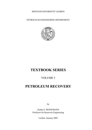
Fig.1.1 shows the life cycle of a reservoir, and the range of recovery estimates.
PERIOD AB:
When no well is drilled, any estimate will be supported by the analogous method based
on data from similar pools. In this phase probabilities of the
• presence of a trap,
• presence of oil or gas saturation,
• presence of pay and
• amount of recoverable reservoir contents
have to be estimated. No reserves is a real option.
PERIOD BC:
The field is being discovered and step by step developed. The production rate increases.
The volumetric estimation can be made more and more precise due to the increasing
Npmax Np or Gpmax– Gp–
ER
CumulativeProduction
O.O.I.P.
-------------------------------------------------------------
Np
N
------ or ER
Gp
G
-------===
ERmax
Ultimate Recovery
O.O.I.P.
--------------------------------------------------
Npmax
N
--------------- or ERmax
Gpmax
G
----------------===
17. Chapter 1: Introduction 3
number of wells available.
PERIOD CD:
The field has been developed and the production rate achieved a maximum. The majority
of possible informations from
• well logs
• core analysis and
• transient well testing
are available. The volumetric estimation can be made more precise when analysing the
reservoir performance. Early simulation studies, called reservoir modeling, make the
calculation of the ultimate recovery possible.
PERIOD DE:
The recovery mechanisms are well known. Material balance calculations and simulation
of the reservoir history provide, in most of the cases, more accurate figures of O.O.I.P.
than the volumetric method. These methods are more suited to compute the reserves than
the volumetric method.
PERIOD EF:
In addition to material balance calculations and simulation studies decline curve analysis
becomes more appropriate.
18. 4 Chapter 1: Introduction
Figure 1.1: Range in estimates of ultimate recovery during the life of a reservoir
Property Status
Study Method
Pre-drilling
Period
Analog
1
Well
Completed
st
B C D E FA
B C D E FA
Production Operations
AbandonmentDevelopment
Period
Range of Estimates
Volumetric
Performance
Simulation Studies
Material Balance Studies
Decline Trend Analyses
Actual Recovery
Range of Recovery Estimates
Production Profile
UltimateRecovery
Cumulative
Rate
LogProductionRate
CumulativeProduction
Risk
High
Low
Relative Risk Time
19. Chapter 1: Introduction 5
1.2 Classification of Reserves
Reserves are divided into classes. The definition of these classes is not common in all
countries. Here the recommended nomenclature system of MARTINEZ et al.[28.](1983)
published at the 11th
World Oil Congress, London, is used.
PROVED RESERVES of petroleum are the estimated quantities, as of a specific date,
which analysis of geological and engineering data demonstrates, with reasonable
certainty, to be recoverable in the future from known reservoirs under the economic and
operational conditions at the same date.
PROVED DEVELOPED RESERVES are those proved reserves that can be expected to be
recovered through existing wells and facilities and by existing operating methods.
Improved recovery reserves can be considered as proved developed reserves only after an
improved recovery project has been installed.
PROVED UNDEVELOPED RESERVES are those proved reserves that are expected to be
recovered from future wells and facilities, including future improved recovery projects
which are anticipated with a high degree of certainty.
UNPROVED RESERVES of petroleum are the estimated quantities, as of a specific date,
which analysis of geological and engineering data indicate might be economically
recoverable from already discovered deposits, with a sufficient degree of certainty to
suggest the likelihood or chance of their existence. Unproved reserves may be further
categorized as PROBABLE RESERVES where there is a likelihood of their existence, or
POSSIBLE RESERVES where there is only a chance of their existence. The estimated
quantities of unproved reserves should take account of the uncertainties as to whether, and
to what extent, such additional reserves may be expected to be recoverable in the future.
The estimates, therefore, may be given as a range.
SPECULATIVE RESERVES of petroleum are the estimated quantities, as at a specific
date, which have not yet been discovered, but which general geological and engineering
judgement suggests may be eventually economically obtainable. Due to the great
uncertainties, they should always be given as a range.
21. 7
7
Chapter 2
Reserves Calculation by Volumetric
Methods
2.1 Computation of Oil and Gas in Place
The following formulas are used:
OOIP - Original oil in place:
(2.1)
OGIP - Free gas in a gas reservoir or in a gas cap:
(2.2)
Solution gas in an oil reservoir:
(2.3)
where
V - reservoir volume [m3]
φ - porosity [-]
Swi - initial water saturation [-]
N
Vφ 1 Swi–( )
Boi
-----------------------------.=
GF
Vφ 1 Swi–( )
Bgi
-----------------------------.=
Gs
Vφ 1 Swi–( )Rsi
Boi
------------------------------------- NRsi,==
22. 8 Chapter 2: Reserves Calculation by Volumetric Methods
The reservoir volume V can be calculated in different ways. Which method is the best
depends on the available data, shape of the reservoir, etc..
2.2 Recovery Factor
Ultimate recovery is influenced by a lot of individual physical realities. It depends on the
• drive mechanism of the reservoir,
• mobility of reservoir fluids,
• permeability and variation of permeability, both vertically and in the area,
• inclination and stratification of the layers,
• strategy and methods of field development and exploitation.
In the exploration and early exploitation stage, only analogous or statistical methods can
be used to estimate the ultimate recovery factor. It is necessary to examine known
reservoirs from the same region.
ARPS et al.[2.] examined a large amount of oil fields with depletion drive and with water
drive. The results were published by the American Petroleum Institute. The formulas are
known as API formulas for estimation of the ultimate recovery factor.
Depletion or gas drive:
(2.4)
Water or gravitation drive:
(2.5)
where is the initial pressure, the abandonment pressure, and the bubble point
pressure. The subscripts i and b denote that the value is valid at or . The numerical
results of the API examination are summarized in Table 2.1.
Boi - oil formation volume factor (FVF) at initial pressure [m3
/sm3
]
Bgi - gas formation volume factor at initial pressure [m3
/sm3
]
Rsi - initial solution (or dissolved) gas oil ratio [sm3
/sm3
]
ER %( ) 41.815
φ 1 Sw–( )
Bob
-----------------------
×
0.1611
k
µob
--------
0.0979
Sw
0.3722
pb
pa
-----
0.1714
=
ER %( ) 54.898
φ 1 Sw–( )
Boi
------------------------
0.0422 k
µoi
-------µwi
0.077
Sw
0.1903– pi
pa
-----
0.2159–
=
pi pa pb
pi pb
23. Chapter 2: Reserves Calculation by Volumetric Methods 9
Table 2.1: API Ultimate Recovery Factor Estimation
2.3 Data Distribution and Probability
The methods for calculation of the reservoir volume, average porosity and permeability
are subjects of reservoir geology and log evaluation. These data are more or less uncertain
and have to be treated as random variables.
Interpretation of even moderately large amounts of data requires statistical methods. A
commonly used method is to gather individual data into groups or classes. This facilitates
interpretation as well as numerical computations. Porosity data are used to demonstrate
this ascertainment. An example of raw data is given in Table 2.2.
Table 2.2: Porosity Sample Data (n=24 values)
Class boundaries, as given in Table 2.3, coincide in terms of the upper boundary of one
class being the same as the lower boundary of the next class. Common convention is to
take the values at the boundary into the higher class. The difference between upper and
lower boundaries is referred to as the class interval. Normally but not necessarily, the class
intervals are equal.
Average porosity can be calculated either from the data in Table 2.2 or in Table 2.3:
(2.6)
Standard
deviation
Sand, Sandstone
min. mean max.
Carbonates
min. mean max.
Depletion +
Gasdrive
0.229 0.095 0.213 0.460 0.155 0.176 0.207
Water or
Gravitationdrive
0.176 0.131 0.284 0.579 0.090 0.218 0.481
0.165 0.198 0.196 0.185 0.192 0.188
0.187 0.184 0.182 0.205 0.178 0.175
0.192 0.205 0.162 0.162 0.182 0.170
0.184 0.165 0.154 0.179 0.172 0.156
Σx = 4.317
φ
xj
j 1=
n
∑
n
--------------
4.317
24
------------- 0.1798== =
24. 10 Chapter 2: Reserves Calculation by Volumetric Methods
(2.7)
It is evident that
(2.8)
Table 2.3: Frequency Distribution
Histograms and frequency polygons are used to show the probability density. Fig. 2.1
shows both of them for the porosity data included in the foregoing tables. The frequency
polygon is drawn through the midpoints of the classes. The areas below the histogram and
the frequency polygon are equal.
The cumulative frequency polygons are shown in Fig. 2.2. Based on this diagram, one can
conclude that 60% of the samples have a porosity less than about 18.5%. Two important
statistical properties of the data group are
the variance
(2.9)
and the standard deviation
(2.10)
Class
Boundaries
Members
Frequency
fi
Class Mark
xi
fi.xi
0.15-0.16 0.156, 0.157 2 0.155 0.311
0.16-0.17 0.162, 0.162, 0.165, 0.165 4 0.165 0.660
0.17-0.18 0.170, 0.172, 0.175, 0.178, 0.179 5 0.175 0.875
0.18-0.19 0.181, 0.182, 0.182, 0.184, 0.185, 0.187 7 0.185 1.295
0.19-0.20 0.192, 0.192, 0.196, 0.198 4 0.195 0.780
0.20-0.21 0.205, 0.205 2 0.205 0.410
24 4.330
φ
*
fix
i
i 1=
n
∑
fi∑
------------------
4.33
24
---------- 0.1804== =
φ φ
*
n ∞→
lim=
σ
2
xj x–( )
j 1=
n
∑
n
-----------------------------------
2
=
σ
xj x–( )
j 1=
n
∑
n
-----------------------------------
2
=
25. Chapter 2: Reserves Calculation by Volumetric Methods 11
Figure 2.1: Histogram for porosity data (Table 2.3)
Figure 2.2: Cumulative frequency of porosity data (Table 2.3)
For the foregoing example, these are
; . (2.11)
The local maximum of the probability density is called the modus. If the distribution is
symmetrical, the modus is equal to the mean value.
0.14
Porosity
Frequency
Relativefrequency
2
4
6
8
0
0.1
0.2
0.3
0.180.16 0.20 0.22
0.14
Porosity
Cumulativefrequency
Cum.relativefrequency
0.25
0.50
0.75
1.00
0
0.180.16 0.20 0.22
6
12
18
24
0
σ
2
φj φ–( )
j 1=
n
∑
n
------------------------------------
2
0.0002== σ 0.014=
26. 12 Chapter 2: Reserves Calculation by Volumetric Methods
2.3.1 Triangular Distribution
In the majority of practical cases, it is not possible to get a reliable histogram or frequency
polygon. One has to be content with estimating the upper, the lower and the modus.
For the data given in Table 2.2 the following estimation would be possible:
, , , . (2.12)
Fig. 2.3 illustrates the triangular distribution of this data. The height of the triangle is
selected in a way so that the surface value becomes 1. The probability that the value (φ)
will be less than the modes (φmod) is
(2.13)
and 1 - p that it will be higher. The cumulative probability can be calculated as follows:
, , (2.14)
, . (2.15)
The variance is
. (2.16)
Fig. 2.4 shows the F-function for the triangular probability distribution in Fig. 2.3. It is
very similar to the diagram in Fig. 2.2. In fact, cumulative relative frequency and
cumulative probability have the same meaning.
φmin 0.150= φmax 0.210= φmod 0.185= φ 0.180=
p
φmod φmin–
φmax φmin–
------------------------------=
F p
φ φmin–
φmax φmin–
-----------------------------
2
= φmin φ φmod≤ ≤
F 1 1 p–( )
φmax φ–
φmax φmin–
-----------------------------
2
–= φmod φ φmax≤ ≤
σ
φmax φmin–( )
2
18
------------------------------------- 1 p 1 p–( )–[ ]=
27. Chapter 2: Reserves Calculation by Volumetric Methods 13
Figure 2.3: Triangular probability distribution
Figure 2.4: Cumulative probability calculated from Fig. 2.3
2.3.2 Uniform Distribution
An uniform distribution is illustrated in Fig. 2.5. The randomly occurring values are
evenly distributed in the range from minimum to maximum values. The cumulative
probability is defined by:
, . (2.17)
For φ = φmin, F = 0 and for φ = φmax, F = 1.
0.14
Porosity
Probability
0.16 0.20 0.22
0.20
0.10
0.30
0
Φmod ΦmaxΦmin
0.18
0.14
Porosity
0.180.16 0.20 0.22
0
0.25
0.50
0.75
1.0
Cumulativeprobability
F p φ( ) φ
φ φmin–
φmax φmin–
-----------------------------=d
φmin
φmax
∫= φmin φ φmax≤ ≤
28. 14 Chapter 2: Reserves Calculation by Volumetric Methods
The variance is
. (2.18)
Figure 2.5: Uniform probability distribution
2.3.3 Dependent Distribution
Reservoir data applied for computation purposes of the reservoir are not independent. For
example, the water saturation may be calculated from the ARCHIE[1.]
formulas:
(2.19)
(2.20)
thus
(2.21)
where
Rw - the connate water resistivity Ωm [Ωft],
Rt - the formation resistivity Ωm [Ωft],
F - the formation factor,
a, m, n - positive constants.
σ
2 φmax φmin–( )
2
12
-------------------------------------=
0.14
Porosity
0.180.16 0.20 0.22
0
0.25
0.50
0.75
1.0
Probability
0
0.25
0.50
0.75
1.0
Cumulativeprobability,F
F aφ
m–
=
Rt FRwSw
n–
=
Sw
aRw
Rt
----------
1
n
---
φ
m
n
----–
=
29. Chapter 2: Reserves Calculation by Volumetric Methods 15
It is evident, that Sw increases if φ decreases. Fig. 2.6 shows such a dependence for a
triangular distribution of the connate water saturation.
Figure 2.6: Use of dependent distribution
2.4 Monte Carlo Simulation Method
Calculate the following formula:
. (2.22)
x and y are stochastic variables. Their cumulative probabilities between their minimum
and maximum values are known. The task is to determine the probability distribution and
the expected value of z.
The computation is simple, but less suitable for hand calculations than for the computer.
For calculations it is necessary to use a random number generator.
Values entering into Eq. 2.22 are repeatedly selected by random numbers taken from an
appropriate range of values, as it is shown in Fig. 2.7. Within several hundred to several
thousand trials, the number of z values for prefixed classes are counted. The result is a
histogram and the cumulative relative frequency for the z variable.
0
Connate water saturation
0.5 1.0
0.10
0.15
0.20
0.25
0.30
Porosity
min
m
odusm
ax
z xy=
30. 16 Chapter 2: Reserves Calculation by Volumetric Methods
Figure 2.7: Selecting random values from a triangular distribution
(after McCray, 1975)
Example 2.1
Calculating the porosity and water saturation (Sw) from well logs (after Walstrom et
al.[39.](1967).
The calculation steps are as follows:
1. Determine φ from the relation:
.
2. Use the value of to determine formation factor F from the Archie formula:
.
3. Use the value of F and randomly chosen values of other quantities to determine Sw
from the relation
,
Value of parameter
0
0
1.0
Cumulativeprobability
orfrequency
xmin xmax 1.0
xmin xmaxxmod
Probability
density
Uniform
distribution
Randomnumbers
0
1
φ( )
ρB ρFφ ρ+ Ma 1 φ–( )=
φ
F aφ
m–
=
Rt FRwS
n–
w
=
31. Chapter 2: Reserves Calculation by Volumetric Methods 17
where
The range of parameter used in this example is given in Table 2.4. Uniform distribution
was assumed for all quantities, except parameters a and ρF, which where assumed to be
constants. The results of the simulation are shown in Fig. 2.8, Fig. 2.9 and Fig. 2.10, these
reflect the results of several hundred cases, wherein each case was processed through
steps 1, 2 and 3. Here it may be noted that although uniform distribution was assumed for
quantities entering the calculations, the resulting probability densities are not
symmetrical. The functional relationship of the quantities may skew the results.
Table 2.4: Ranges of Parameters Used in a Log-Interpretation Example
(metric units)
ρB - the bulk density kg m-3[1b/cuft],
ρF - the fluid density kg m-3
[1b/cuft],
ρMa - the rock matrix density kg m-3[1b/cuft],
Rw - the connate water resistivity Ωm [Ωft],
Rt - the formation resistivity Ωm [Ωft],
F - the formation factor,
a, m, n - positive constants.
Parameter Lower Limit Upper Limit
Rt True resistivity Ωm 19.000 21.000
Rw Connate water resistivity Ωm 0.055 0.075
n Exponent in the ARCHIE equation 1.800 2.200
a Coefficient in the ARCHIE equation 0.620 0.620
m Exponent in the ARCHIE equation 2.000 2.300
ρB Bulk density kg/m3 2.360 2.380
ρMA Rock mineral density kg/m3 2.580 2.630
ρF Reservoir fluid density kg/m3 0.900 0.900
32. 18 Chapter 2: Reserves Calculation by Volumetric Methods
Table 2.5: Ranges of Parameters Used in a Log-Interpretation Example
(field units)
Figure 2.8: Calculated porosity (after Walstrom et al. 1967)
Parameter Lower Limit Upper Limit
Rt True resistivity Ωft 62.300 68.900
Rw Connate water resistivity Ωft 0.180 0.246
n Exponent in the ARCHIE equation 1.800 2.200
a Coefficient in the ARCHIE equation 0.620 0.620
m Exponent in the ARCHIE equation 2.000 2.300
ρB Bulk density lb/cu ft 147.300 148.600
ρMA Rock mineral density lb/cu ft 161.000 164.200
ρF Reservoir fluid density lb/cu ft 56.200 56.200
0.10
Porosity
0.140.12 0.16 0.18
0
0.10
0.20
0.30
0.40
0.50
Probability
33. Chapter 2: Reserves Calculation by Volumetric Methods 19
Figure 2.9: Formation factor (after Walstrom et al. 1967)
Figure 2.10: Calculated water saturation (after Walstrom et al. 1967)
Example 2.2
Calculation of oil recovery
The ultimate recovery was estimated by combination of the Eq. 2.1 and Eq. 2.5:
(2.23)
Symmetric triangular distribution was assumed for all the quantities in Eq. 2.23, except
the parameter which is constant 0.7 cP. The limits are shown in Table 2.6 and Table
2.7.
The ultimate recovery from this reservoir can be characterized with the following figures
26
Formation factor
Probability
0.05
0.10
0.15
0.20
0
34 42 50 58 66 74 8218
24
Water saturation
3630 42 48 54 60
Probability
0.20
0.10
0.30
0
Npmax NER 0.54898V
φ 1 Sw–( )
Boi
-----------------------
1.04222 kµwi
µoi
-----------
0.077
Sw
0.1903– pi
pa
-----
0.2159–
==
µwi
34. 20 Chapter 2: Reserves Calculation by Volumetric Methods
of a Monte Carlo simulation with 5000 trials.
Probability distribution:
Taking for all parameters the most unfavorably and the most favorably the following
realistically figures can be calculated:
Table 2.6: Range of Parameters Used in the Ultimate Recovery Calculation Example
(metric units)
Expected ultimate recovery: 16,540,000 m3
or 104.03 MMbbl
with standard deviation of: 1,100,000 m3 or 6.91 MMbbl
with more than but less than
99% 13.82 - 19.24.103m3 [86.9 - 121.0 MMbbl]
90% 14.70 - 18.38.106m3 [92.4 - 115.6 MMbbl]
80% 15.08 - 18.00.106
m3
[94.8 - 113.2 MMbbl]
Worst case: Best case:
12.227x10⁶ m3 21.726x10⁶ m3
(76.9x10⁶ bbl) (136.6x10⁶bbl)
Parameter Unit Lower Limit Upper Limit
V Reservoir volume 106
m3
285.000 370.00
φ Porosity 0.165 0.19
Sw Initial water saturation 0.220 0.28
Boi Formations volume factor 1.480 1.50
µoi Reservoir oil viscosity cP 2.850 2.95
k Reservoir permeability darcy 0.800 1.50
pi Initial pressure (pi = pb) MPa 22.000 22.50
pa Abandonment pressure MPa 18.000 20.00
35. Chapter 2: Reserves Calculation by Volumetric Methods 21
Table 2.7: Range of Parameters Used in the Ultimate Recovery Calculation Example
(field units)
Figure 2.11: Ultimate recovery calculation with Monte Carlo simulation
Parameter Unit Lower Limit Upper Limit
V Reservoir volume 105
ac ft 2.310 3.000
φ Porosity 0.165 0.190
Sw Initial water saturation 0.220 0.280
Boi Formations volume factor 1.480 1.500
µoi Reservoir oil viscosity cP 2.850 2.950
k Reservoir permeability mD 800.000 1.500
pi Initial pressure (pi = pb) psi 3.190 3.262
pa Abandonment pressure psi 2.610 2.900
Cumulative distribution 10 [m ]
6 3
13.5 16.5
Cell C10
15.0 18.0 19.5
0.25
0.50
0.75
1.00
0 0
4985
Probability
Frequency
36. 22 Chapter 2: Reserves Calculation by Volumetric Methods
37. 23
23
Chapter 3
Material Balance
3.1 Tarner’s Formulation
Fig. 3.1 shows a schematic illustration of an oil reservoir. The rock volume is V and the
porosity φ. Apart from a certain saturation of connate water Swi, the rock is saturated with
hydrocarbons. Thus, the effective reservoir volume is
. (3.1)
The reservoir temperature is defined as T, the initial pressure as pi. The virgin reservoir is
in a state of hydrostatic and thermodynamic equilibrium.
The original oil in place is defined as N in sm3 or stb (stock tank barrels). At reservoir
conditions gas is dissolved in the oil. The amount is expessed by the initial solution GOR
(gas-oil ratio) Rsi sm3
/sm3
or scft/stb.
The formation volume of the oil is NBoi. If the reservoir contains the same or a greater
amount of gas than soluble at reservoir conditions (pressure and temperature), the
reservoir is saturated and the surplus gas forms a gas cap. Otherwise, the reservoir is
undersaturated.
Should the gas cap contain an amount of G sm3
or scft gas, then its formation volume will
be GBgi. Usually the volume of the gas cap is expressed in relation to the oil volume:
. (3.2)
Vφ 1 Swi–( ) VP 1 Swi–( )=
GBgi mNBoi=
38. 24 Chapter 3: Material Balance
When regarding surface and formation volumes the following relations can be set up:
Figure 3.1: The scheme of the material balance of an oil reservoir
The effective pore volume, expressed by the amounts of oil and gas, is:
. (3.3)
After a certain time period, an amount of
Fluid Surface Formation
Oil N sm3
[stb] NBoi m3[bbl]
Dissolved Gas NRsi sm3[scft] --
Free Gas GF sm3[scft] GFBgi = mN Boi m3[cuft]
Oil Np sm3
[stb],
Gas Gp=NpRp sm3 [scft],
Water Wp sm3
[bbl]
Initial reservoir pressure: p
net pore volume: VF(1-S )
i
wi Reservoir content
GB +g
NBoi
Expanded reservoir volumes
Production in reservoir volumes
At reservoir pressure p
GBg
N (R -R )Bp p s g
Wo
Wp
N Bp o
NB +NB (R -R )o g si s
+NB (R -R )-
-N B (R -R )
g si s
p g si s
(N-N )Bp o
W -Ws p
GB =mNBgi oi
NBoi GBgi+ VP 1 Swi–( )=
39. Chapter 3: Material Balance 25
will have been produced. Rp is the cumulative production GOR. As a consequence of
production, the reservoir pressure decreases from pi to p.
Figure 3.2: Pressure drop and production of a reservoir
Let us now consider the reverse situation. At first pressure drops to p. Thus, the gas cap
expands and gas evolves from the oil. From the aquifer an amount of We water will flow
into the reservoir. The expanded system would have a reservoir volume at pressure p of
. (3.4)
At the same pressure the produced fluids would have a total reservoir volume of
. (3.5)
The effective pore volume corresponding to Eq. 3.1 remains unchanged which
consequently makes the following assertion valid:
[expanded volume] - [initial volume] = [produced volume]
or
Eq. 3.4 - Eq. 3.3 = Eq. 3.5
Production time [month]
Cumulativeproduction
NandW10[m]PP
33
Rm/mp
33
40
60
80
100
Reservoirpressure[mPa]
16
18
20
22
24
26
0
200
400
600
800
1000
0 24 48 72 96 120 144
Past
RP
WP
NBo mNBoi
Bg
Bgi
-------- NBg Rsi Rs–( ) We+ + +
NpBo NpBg Rp Rs–( ) Wp+ + Np Bo Bg Rp Rs–( )+[ ] Wp+=
40. 26 Chapter 3: Material Balance
After substituting:
(3.6)
From this
. (3.7)
This is the formula of TARNER’s[37.]
material balance. If in addition to production, water
is injected at the cumulative amount of WI and/or gas at the cumulative amount of GpI,
then the term (WI + GpIBg) has to be added to the numerator. I indicates how much of the
produced gas was reinjected into the reservoir.
Every specific term in Eq. 3.7 has a certain meaning:
(3.8)
Eq. 3.6 is then divided by Bg
(3.9)
N Bo Boi–( ) N mBoi
Bg
Bgi
-------- 1–
Bg Rsi Rs–( )+ We+ +
Np Bo Bg Rp Rs–( )+[ ] Wp+=
N
Np Bo Bg Rp Rs–( )+[ ] We Wp–( )–
mBoi
Bg
Bgi
-------- 1–
Bg Rsi Rs–( ) Boi Bo–( )–+
--------------------------------------------------------------------------------------------------------=
N
−+
−−
=
gas cap expansion
43421
Bg
Bgi
mBoi
reservoir oil
shrinkage
( )
43421
−Boi Bo
desoluted gas
expansion
(
4434421
−Rsi Rs)Bg
net water influx
( )−+ WpWIWe
injected gas
G BI g
produced hydrocarbons
( )[
444 8444 76
−+ RsRpBgBo ]Np
Reservoir volume of
41. Chapter 3: Material Balance 27
Eq. 3.9 is divided by its right hand side:
(3.10)
3.2 Drive Indices
Splitting up the left side of Eq. 3.10 leaves three fractions which describe the shares of the
specific drive mechanisms in reference to the whole cumulative production effected by
• the solution gas drive,
• the gas drive and
• the water drive.
These are considered the drive indices. The solution gas drive index (a two phase
expansion of the oil) is defined as
. (3.11)
The gas drive index (expansion of the gas cap) is defined as
. (3.12)
The water drive index (expansion of the aquifer) is defined as
. (3.13)
N
Bo
Bg
------ Rs–
Boi
Bg
-------- Rsi–
– mNBoi
1
Bgi
--------
1
Bg
------–
1
Bg
------ We Wp–( )+ +
Np
Bo
Bg
------ Rs–
NpRp+
------------------------------------------------------------------------------------------------------------------------------------------------------------ 1=
Is
N
Bo
Bg
------ Rs–
Boi
Bg
-------- Rsi–
–
Np
Bo
Bg
------ Rs–
NpRp+
-------------------------------------------------------------------=
Ig
mNBoi
1
Bgi
--------
1
Bg
------–
Np
Bo
Bg
------ Rs–
NpRp+
--------------------------------------------------=
Iw
1
Bg
------ We Wp–( )
Np
Bo
Bg
------ Rs–
NpRp+
--------------------------------------------------=
42. 28 Chapter 3: Material Balance
The relation between the indices is given by
. (3.14)
Cumulative oil-, gas- and water production (Np, Rp, Wp) are given by production statistics.
The PVT-properties (Bo,Bg,Rs) are determined by laboratory measurement or by
correlations. The volumetric reserve calculation covers the petroleum in place (N, G). The
average reservoir pressure is recorded by regular measurements of static well bottom-hole
pressures. The application of these data enables a sufficient description of the water influx
as a function of time.
3.3 Water Influx
Operating a reservoir over years, the cumulative oil, gas and water production Np(t), Gp(t),
and Wp(t) are naturally known. The reservoir pressure declines and the actual values p(t)
will be determined by regulare pressure surveys. The fluid properties, as Bo(p), Bg(p) and
Rs(p), are messured in PVT Labs or determined from different types of charts, e.g.: from
Standing correlation. Also the OOIP (N) and the gas cap factor m can be estimated by
volumetric calculation (see Chapter 3.).
The only quantity in Eq. 3.6, which is entierly unknown, is the water influx We(t). The
Material Balance calculation is the only method which enables to determine it as function
of time. From Eq. 3.6:
(3.15)
The aquifer is a water bearing formation, hydrodynamically connected to the hydrocarbon
reservoir. Its form, size and permeability can vary greatly. Hydrological reflection could
help to set up hypotheses. However, these can never be verified in detail since no wells
will be drilled to explore an aquifer.
One of the boundaries of the aquifer is the water-oil-contact (WOC). This interior
boundary is usually well known, whereas the exterior boundary is an object of
speculation.
The exterior boundary can be considered closed if the whole amount of water flowing into
the reservoir is due to the expansion of the aquifer. In this case, the aquifer is finite closed.
Faults and layer pinch outs form such boundaries.
Is Ig Iw+ + 1=
We t( ) Np Bo Bg Rp Rs–( )+[ ]
N– Bo Boi– mBoi
Bg
Bgi
-------- 1–
Bg Rsi Rs–( )+ + Wp+
=
43. Chapter 3: Material Balance 29
The aquifer can be considered a finite open one, if the pressure at the exterior boundary is
constant. A connection to the atmosphere through outcropping or hydrodynamic contact
to a karstic formation are the possibilities to form such boundaries. Fig. 3.4 shows a
schematic illustration of an aquifer.
Figure 3.3: Cumulative drive indices
Figure 3.4: Oil reservoir with an aquifer
The cumulative water influx is calculated from the rate:
. (3.16)
Production induces pressure decline at the interior boundary of the aquifer. Let us make a
theoretical consideration. We assume a unique and sudden pressure drop ∆p = pi - p at this
Production time [month]
Cumulativedriveindices
0
0.2
0.4
0.6
0.8
1.0
0 24 48 72 96 120 144
Past PrognosisIg
Is
Iw
Oil
Aquifer
Fault (tectonic boundary)
Inner
WOC
Marl
AquiferReservoir
Water
Outer water-oil-contact
(WOC)
We t( ) q t( )
o
t
∫ dt=
44. 30 Chapter 3: Material Balance
boundary, where pi is the initial reservoir pressure. The pressure drop will cause water
intrusion into the reservoir. Initially, this is a consequence of the expansion of water and
rock and it is independent of the distance to the exterior boundary and regardless of
whether the boundary is closed or not. The depression zone stretches with time - either
fast or slowly, dependent on permeability - whereby the water influx rate permanently
decreases. This situation is given until the depression radius reaches the exterior
boundary. We call this time interval as transient period.
In case of a closed exterior boundary, water influx decreases rapidly and tends to zero, if
the pressure in the whole aquifer has dropped by ∆p. In this case, the function of the
cumulative water influx We(t) has an asymptotic value (see Fig. 3.5).
Figure 3.5: Cumulative water influx at a constant reservoir pressure
If there is an aquifer with constant pressure at the exterior boundary, a stabilization of the
influx rate takes place and therefore the function We(t) becomes linear with increasing
time.
If the aquifer is small or the permeability high, the transient period becomes short and can
be neglected. Under this consideration we distinguish between three types of aquifer
models or water influxes:
1. Semi-steady-state,
2. Steady-state,
3. Non-steady-state:
3.1. Transient
3.2. Pseudo-steady-state.
3.3.1 Semi-Steady-State Water Influx
Sometimes the cumulative water influx can be considered solely as a function of the
Time
Cumulativewaterinflux,We
t
∆p=p-p=constanti
p =pe i
Finite aquifer with
constant pressure
on the boundary
1)
1)
Infinite aquifer
Finite closed aquifer
2)
2)
3)
3)
r =e
p
r
( )r=re
=0
45. Chapter 3: Material Balance 31
pressure drop. That means, the time in which the pressure change took place has no
influence on the intruded water amount, consequently Eq. 3.16 becomes:
. (3.17)
In such a case the aquifer has always a limited size and a closed external boundary. The
coefficient C1 can be expressed by the parameters of the aquifer:
(3.18)
Figure 3.6: Change in reservoir pressure
3.3.2 Steady-State Water Influx
In case of a constant pressure at the exterior boundary and high aquifer permeability the
transient period can be neglected. This is equivalent to the assumption of incompressible
water inside the aquifer. Thus the water influx rate is proportional to the pressure
difference between the two boundaries:
(3.19)
The cumulative water influx is calculated by integration:
(3.20)
This is the SCHILTHUIS[35.]-formula (1936). The coefficient C2 is calculated by
DARCY’s law with the help of the specific aquifer parameters. In the case of linear
We C1 pi p t( )–[ ]=
C1 Ahφce=
∆p0
pi
p1
p2
p3
p4
t4t1 t2
Time, t
t3
Reservoirpressure
∆p1
∆p2
∆p3
q t( ) C2 pi p t( )–[ ]=
We t( ) C2 pi p t( )–[ ] td
o
t
∫=
46. 32 Chapter 3: Material Balance
aquifers (Fig. 3.7)
, (3.21)
where
Figure 3.7: Idealized aquifers
In the case of radialsymmetric aquifers (Fig. 3.7 B), the coefficient is:
, (3.22)
where replace 2π by 7.08 x 10 -3
for field units to get [bbl/psi d]. There are
The pressure p(t) in Eq. 3.20 is the pressure at the inner boundary. In most of the practical
cases it will be replaced by the average reservoir pressure, given for discrete time points:
to = 0, t1, t2, ...., tn. Although this pressure can be plotted with a smooth continuous line,
it is more practical to approximate it with a step function or with linear functions as shown
in Fig. 3.6. For Eq. 3.20 both approximations give the same results.
b - width of the aquifer,
h - thickness of the aquifer,
L - length of the aquifer,
k - permeability of the aquifer,
µ - viscosity of the water.
rw - inner radius,
re - outer radius of the aquifer.
C2L
bhk
µL
---------=
b
h
L
A) B)
rw
re
C2r
2πhk
µ
re
rw
-----ln
---------------=
47. Chapter 3: Material Balance 33
(3.23)
3.3.3 Non-Steady-State Water Influx
Usually the water influx has non-steady-state character. We distinquish between transient
and pseudo-steady state flow regime. Note that both are non-steady state flow.
The theoretical funded and general applicable method, covering transient,
pseudo-steady-state and steady-state flow as well, was published by van Everdingen and
Hurst[16.]
(1949). The method was slighly modified by Vogt and Wang[41.]
(1988), making
it more convenient for computer programming. The derivation was discussed in the
Volume 1 of this Textbook series (Heinemann, Z.E.: "Fluid Flow in Porous Media",
Chapter 3). We use the Vogt-Wang formulation as our standard method.
Under pseudo steady state conditions the water influx results from the uniform expansion
of the aquifer, which means that the rate of pressure change is equal in the whole aquifer
domain.
3.3.3.1 Vogt-Wang Aquifer Model
It was assumed that the reservoir area can be approximated by a segment of a circle. The
radius is
, (3.24)
where ω is the arc in radian (= 2π for complete circle) and re is the outer radius of the
aquifer.
The dimensionless outer radius is
. (3.25)
We t( ) C2 pi p t( )–[ ]
tj 1–
tj
∫
j 1=
n
∑ dt=
We t( ) C2 pi
pj pj 1–+
2
-----------------------–
j 1=
n
∑ tj tj 1––( )
We t( ) C=
2
pi pj–( )
j 1=
n
∑ tj tj 1––( )
=
rw
2A
ω
-------
1 2⁄
=
reD
re
rw
-----=
48. 34 Chapter 3: Material Balance
The dimensionless time is
(x 0.00634 for field units, t in days). (3.26)
The cumulative water influx at the time tDj is
(3.27)
The functions are given in Table 3.1 only for an infinite acting radial aquifer. In
case of finite aquifers we refer to the paper of VOGT and WANG[41.](1988).
In radial symmetrical homogeneous case the coefficient C3 can be calculated as
(x 0.1781 for bbl/psi). (3.28)
Example 3.2 - Example 3.4 demonstrate how the coefficients C1-C3 and the function We(t)
are calculated.
Usually the aquifer parameters are unknown. It is possible however (as shown in Example
3.1) to determine the water influx of the past with help of the material balance equation.
First it is essential to ascertain the semi-steady-state, steady state or non-steady-state
character of the water influx.
Example 3.1 is continued by Example 3.5. If either C1 nor C2 is a constant but the
coefficient C1 calculated at various times increase steadily whereas C2 continuously
decreases, coefficient C3 can be determined with sufficient accuracy. The dispersion of
the C3-values indicates how appropriate reD and α were chosen. If α is too small, the
function
(3.29)
is not linear, but has an upward curvature. If α is too big, the curvature is directed
downwards. Only numerous repetitions of the calculation using various values of reD
provide a favorable solution.
tD
k
φµwcerw
2
----------------------t αt==
Wej C3
po p1–
tD1
-----------------Q˜ tDj( )
p1 p2–
tD2 tD1–
----------------------
po p1–
tD1
-----------------–
Q˜ tDj tD1–( )...
+
pj 1– pj–
tDj tDj 1––
---------------------------
pj 2– pj 1––
tDj 1– tDj 2––
-----------------------------------–
Q˜ tDj tDj 1––( )}
+
=
Q˜ tD( )
C3
id
ωφhcerw
2
=
We f
∆p
∆tD
---------
∆∑ Q˜=
50. 36 Chapter 3: Material Balance
The VAN EVERDINGEN-HURST solution requires the calculation of the sum at every
time tD for every j. This is for limited aquifers not necessary if the early transient period
is over.
3.3.3.2 Fetkovich Aquifer Model
Fetkovich[17.] presented a simplified approach for such cases that utilizes the
pseudo-steady-state aquifer productivity index and an aquifer material balance to
represent a finite compressibility system.
Assuming that the flow obeys DARCY’s law and is at pseudo-steady-state or steady-state,
the generalized rate equation for an aquifer without regarding the geometry can be
written:
. (3.30)
Jw is defined as the productivity index of the aquifer. pwf is the pressure at the inner radius
and p is the average aquifer pressure. The later value can be calculated from a material
balance for a constant compressibility:
, (3.31)
where W is the water content and ce = cw + cφ the total compressibility of the aquifer. The
maximum encroachable water at p = 0 is:
(3.32)
After substituting Eq. 3.32 into Eq. 3.31:
(3.33)
The calculation is reduced to the following steps:
• For a time interval ∆j+1t = tj+1 - tj the constant influx rate would be:
, (3.34)
where pj is the average aquifer pressure for the time tj and pwfj+1 is the average inner
boundary pressure during the period ∆j+1t.
qw Jw p pwf–( )=
p
We
ceW
----------– pi+=
Wei ceWpi=
p
pi
Wei
---------– We pi+=
qw Jw pj pwfj 1+–( )=
51. Chapter 3: Material Balance 37
• The total efflux during the timer interval ∆j+1t would be
(3.35)
• The cumulative efflux to the time ∆j+1t would be:
(3.36)
• The aquifer average pressure for the next time interval:
(3.37)
The efflux of the aquifer is naturally the water influx for the reservoir.
The VAN EVERDINGEN-HURST[16.] method in the original form and in the modified
form by VOGT and WANG[41.] as well uses three parameters: C3, α and reD. The first two
are numerical constants, the third relates to the mathematical assumption of a radial
symmetrical aquifer.
The Fetkovich[17.] method uses only two parameters (Jw and Wei) and no relation was
made to any geometrical form. In spite of that Jw and Wei can be calculated for the radial
symmetric case easily as described in the volume "Fluid Flow in Porous Media":
(3.38)
(3.39)
where f=1 if the circle is in full size. For field units replace 2π by 7.08x10-3 in Eq. 3.38
to get [bbl/psi d]. There Eq. 3.34 - Eq. 3.37 give the exact solution of the time step go to
zero. For practical cases a time step of some months gives results accurate enough.
Example 3.1
An oil reservoir contains N = 3.6 x 10⁶
m3
[2.264x10⁷
bbl] oil. The ratio of the gas-/oil-pore
volume is m = 0.3. The change of the reservoir pressure and the cumulative productions
are given in columns (1)-(5) in Table 3.4 and Table 3.5. Columns (6)-(8) tabulate the
values for Bg, Bo and Rs at the corresponding reservoir pressure. The task is to calculate
water influx.
∆Wej 1+ Wej 1+ Wej– qw∆j 1+ t= =
Wej 1+ Wej ∆Wej 1++ ∆
n 1+
j 1+
∑ Wen= =
pj 1+
pi
Wei
---------Wej 1+ pi+–=
Jw
2πhkf
µ
re
rw
-----
3
4
---–ln
------------------------------=
Wei fπ re
2
r
2
w–( )hcepi=
52. 38 Chapter 3: Material Balance
Solution
From Eq. 3.6:
The routine of the calculation procedure can be set up as follows (the numbers indicate
the column numbers):
The results are written in Column (9)
Example 3.2
Figure 3.4 shows an oil reservoir with a semicircular aquifer. The parameters of the
aquifer are
At the time t = 0 reservoir pressure is reduced by 1 MPa [145 psi] and is then kept
constant. The water influx can be considered steady-state. The cumulative water influx
after 3 years is to be calculated.
rw - 1000 m [3280 ft]
re - 5000 m [16400 ft]
h - 7.2 m [23.6 ft]
φ - 0.23
k - 0.0225x10⁻¹² m2 [~ 22.2 mD]
µw - 0.00025 Pas [0.25 cp]
We Np Bo Bg Rp Rs–( )+[ ]
N– Bo Boi– mBoi
Bg
Bgi
-------- 1–
Bg Rsi Rs–( )+ + Wp+
=
9( ) 3( ) 6( ) 7( ) 4( ) 8( )–( )×+[ ]× N
6( ) Boi mBoi 7( ) Bgi 1–⁄( ) 7 Rsi 8( )–( )×+ +–[ ] 5( )+×
–=
53. Chapter 3: Material Balance 39
Solution
From Eq. 3.22 for the semicircular aquifer:
In field units:
The cumulative water influx after 1000 days totals
In field units:
Example 3.3
The task is to determine cumulative water influx after a production time of t = 1000 days
at non-steady-state conditions (Fig. 3.4). During this time the reservoir pressure is reduced
linear by 1 MPa [145 psi]. The aquifer acting infinite.
The parameters of the aquifer are:
A is the area of the aquifer.
A = 14x106
m2
[3459 ac]
h = 7.2 m [23.6 ft]
φ = 0.23
k = 0.225x10⁻¹²
m2
[~ 222 mD]
cφ = 6x10⁻¹⁰ Pa-1 [4.13685x10⁻⁶ 1/psi]
cw = 5x10⁻¹⁰
Pa-1
[3.4473x10⁻⁶
1/psi]
µw = 0.25x10⁻³
Pas [0.25 cP]
C2r
1
2
---
2πhk
µ
re
rw
-----ln
---------------
π7.2 0.0225 10
12–
××
0.25x10
3–
5ln
------------------------------------------------------ 1.265 10
90–
m
3
Pa
1–
s
1–
C 109.3 m
3
=
×
MPa
1–
d
1–
===
C2r
1
2
---
7.08 10
3–
23.6 22.2×××
0.25 5ln×
------------------------------------------------------------- 4.6095 bbl psi d⁄==
We C2r∆pt 109.3 1× 1000× 109 10
3
× m
3
= = =
We 4.6095 145 1000 677410 bbl=××=
54. 40 Chapter 3: Material Balance
Solution
The radii of the reservoir are
In field units:
The effective compressibility of the aquifer is
In field units:
According to Eq. 3.26:
In field units:
From Table 3.1, at tD = αt = 34.5 we get:
rw
2A
π
-------
1
2
---
28 10
6
×
π
---------------------
2985 m= = =
rw
2 3459× 43560×
π
------------------------------------------
1
2
---
9794 ft==
ce cw cφ+ 6 5+( ) 10
10–
× 1.1 10
9–
× Pa
1–
== =
ce 3.448 10
6–
4.137 10
6–
×+× 7.585 10
6–
× 1 psi⁄= =
α
k
µφcerw
2
---------------------
0.225 10
12–
×
0.25 10
3–
× 0.23× 1.1× 10
9–
× 2985
2
×
-------------------------------------------------------------------------------------------------
α 0.39924 10
6–
s
1–
× 0.0345 d
1–
==
= =
α 6.34 10
3– 222
0.25 10
3–
× 0.23× 7.585× 10
6–
× 9794
2
×
------------------------------------------------------------------------------------------------------- 0.0345 d
1–
=×=
Q˜ tD( ) 380.5562=
55. Chapter 3: Material Balance 41
Eq. 3.28, since the reservoir is semicircular
In field units:
From Eq. 3.26:
In field units:
Example 3.4
A reservoir produces three years. Reservoir pressure has decreased from 30 MPa [4350
psi] to 27 MPa [3915 psi]. The data known are tabulated in columns (1)-(3) in Table 3.4
and Table 3.5. The cumulative water influx after 3 years is to be calculated. The
parameters of the aquifer are the same as in Example 3.3.
Solution
Constants α = 0.0345 d-1 and C3 = 51 000 m3 MPa-1 [2233 bbl/psi] were already
calculated in Example 3.3.
The water influx results in
In field units:
C3
id
πφhcerw
2
π0.23 7.2× 1.1× 10
9–
2985
2
××
C3
id
0.051 m
3
Pa
1–
51000 m
3
MPa
1–
= =
= =
C3
id
0.17801π 0.23× 23.6× 7.585× 10
6–
9794
2
×× 2208 bbl psi⁄==
We C3
id ∆p
tD
-------Q˜ tD( ) 51000 1× 380.5562 34.5 568000=⁄× m
3
==
We 2208 145× 380.5562 34.5⁄ 3.53246 10
6
×=× bbl=
We C3 ∆j 1+
∆p
∆tD
---------
Q˜ tDn tDj–( )=51000 26.189× 1.3356 10
6
× m
3
=
j 0=
n 1–
∑=
We 2208 379.74× 8.38465 10
6
× bbl= =
56. 42 Chapter 3: Material Balance
Example 3.5
A water influx equation for the reservoir in Example 3.1 has to be determined. The radius
of the reservoir is ~ 1000 m [3280 ft], the data of the aquifer are:
Solution
First, it is essential to determine whether the water influx is steady-state or
non-steady-state. The procedure is comprised in Table 3.6 and Table 3.7. The coefficients
C1 and C2 are calculated for all tj by using Eq. 3.17 and Eq. 3.23.
Due to the fact that C1 increases and C2 decreases, the water influx can be considered
non-steady-state.
The aquifer is assumed infinite and α is calculated as follows:
In field units:
In Table 3.8 and Table 3.9, the terms
are calculated for the last three time points. The coefficients C3 are calculated in Table 3.6
and Table 3.7 using Eq. 3.26. The values C3 can be regarded with fair accuracy as
constants during the last 60 months. The value C3 = 5300 m3 MPa-1[230 bbl/psi] can be
accepted for prediction purposes.
φ = 0.23
k = 8x10-15
m2
[8 mD]
ce = 1.1x10⁻⁹
Pa-1
[7.585x10⁻⁶
1/psi]
µw = 0.25x10⁻³ Pas [0.25 cP]
α
k
µφcerw
2
---------------------
8 10
15–
×
0.25 10
3–
× 0.23× 1.1× 10
9–
× 10
6
×
------------------------------------------------------------------------------------------- =
α 1.2648 10
7–
s
1–
× 0.0109 d
1–
1 3month
1–
⁄≈==
= =
α
6.34 10
3–
× 8×
0.23 0.25× 7.585× 10
6–
× 3280
2
×
------------------------------------------------------------------------------------- 0.0190d
1–
1 3⁄( )month
1–
≈==
∆j 1+
j 0=
n 1–
∑
∆p
∆tD
---------
Q˜ tDn tDj–( ), n 1 …6,=
57. Chapter 3: Material Balance 43
Table 3.2: Calculation of Water Influx into an Oil-Reservoir -
Example 3.1 (metric units)
Table 3.3: Calculation of Water Influx into an Oil-Reservoir -
Example 3.1 (field units)
t
month
p
MPa
Np
103m3
Rp
Wp
103m3
Bo Bg Rs
We
103m3
(1) (2) (3) (4) (5) (6) (7) (8) (9)
0 23 1.3032* 0.00480* 97.8* 0.0
6 22 87.8 94.0 0.0 1.2957 0.00502 93.9 5.8
12 21 183.7 92.0 0.1 1.2879 0.00526 90.0 11.1
27 20 308.9 89.0 1.1 1.2800 0.00552 86.0 39.5
48 19 502.8 95.0 3.3 1.2719 0.00581 82.0 166.8
75 18 693.20 99.0 13.2 1.2636 0.00613 77.9 292.2
108 17 905.0 105.0 21.8 1.2550 0.00649 73.8 468.5
t
month
p
psi
Np
103
bbl
Rp
scf/bbl
Wp
103
/bbl
Bo Bg
Rs
scf/bbl
We
103
/bbl
(1) (2) (3) (4) (5) (6) (7) (8) (9)
0 3335 1.3032* 0.00480* 549.2 0
6 3190 552 527 0.0 1.2957 0.00502 527.0 36
12 3045 1155 516 0.6 1.2879 0.00526 505.0 70
27 2900 1943 499 6.9 1.2800 0.00552 483.0 248
48 2755 3162 532 20.7 1.2719 0.00581 460.0 1049
75 2610 4359 555 82.9 1.2636 0.00613 437.0 1837
108 2465 5691 589 136.9 1.2550 0.00649 414.0 2946
62. 48 Chapter 3: Material Balance
3.4 Finite Difference Material Balance Equation
The time is divided into a finite number of optional intervals. At time j, Eq. 3.9 becomes
(3.40)
For time j+1
, (3.41)
where
In order to simplify calculations, the water influx is assumed steady-state.
(Calculations are similar, but more complicated for non-steady-state water influx).
According to Fetkovich[17.]
equation Eq. 3.35,
, (3.42)
where paj is the avarage aquifer pressure at time j and
(3.43)
is the average reservoir pressure in a time period (tj, tj+1). Thus, Eq. 3.40 at time j+1 leads
to
qo - oil production rate m3/d [bbl/d],
qw - water production rate m3
/d [bbl/d],
R - the average production GOR.
N
Bo
Bg
------ Rs–
j
Boi
Bgj
-------- Rsi–
– mNBoi
1
Bgi
--------
1
Bgj
--------–
1
Bgj
-------- Wej Wpj–( )
=Np
Bo
Bg
------ Rs–
j
Gpj+
+ +
Npj 1+ Npj ∆j 1+ Np+ Npj qo∆j 1+ t
Gpj 1+ Gpj R∆j 1+ Np+ Gpj qoR∆j 1+ t
Wpj 1+ Wpj ∆j 1+ Wp+ Wpj qw∆j 1+ t+= =
+= =
+= =
Wej 1+ Wej Jw paj p–( )∆j 1+ t+=
p
pj 1+ pj+
2
-----------------------=
63. Chapter 3: Material Balance 49
(3.44)
From Eq. 3.44 either the production for the time intervall j,j+1
(3.45)
or the duration
(3.46)
can be expressed.
Application of the differential form of MB equation:
N
Bo
Bg
------ Rs–
j 1+
Boi
Bgj
-------- Rsi–
– mNBoi
1
Bgi
--------
1
Bgj 1+
---------------–
1
Bgj 1+
--------------- Wej Wpj–( )
+
1
Bgj 1+
--------------- Jw paj p–( ) qw–[ ]∆j 1+ t
Npj
Bo
Bg
------ Rs–
j 1+
Gpj ∆j 1+ Np
Bo
Bg
------ Rs–
j 1+
R++ +=
+ +
∆j 1+ Np
mNBoi
1
Bgj
--------
1
Bgj 1+
---------------–
N
Bo
Bg
------ Rs–
j 1+
Boi
Bgj 1+
--------------- Rsi–
–+
Bo
Bg
------ Rs–
j 1+
R+
------------------------------------------------------------------------------------------------------------------------------------------------
∆j 1+ Np +
Npj–
Bo
Bg
------ Rs–
j 1+
Gpj–
We Wp–( )
Bgj 1+
--------------------------
Jw paj p–( ) qw–
Bgj 1+
----------------------------------------∆j 1+ t+ +
Bo
Bg
------ Rs–
j 1+
R+
---------------------------------------------------------------------------------------------------------------------------------------------------------=
=
∆j 1+ t
mNBoi
1
Bgj
--------
1
Bgj 1+
---------------–
N
Bo
Bg
------ Rs–
j 1+
Boi
Bgj 1+
--------------- Rsi–
–+
qo
Bo
Bg
------ Rs–
j 1+
R+
Jw paj p–( ) qw–
Bgj 1+
--------------------------------------–
------------------------------------------------------------------------------------------------------------------------------------------------
∆j 1+ t +
Npj–
Bo
Bg
------ Rs–
j 1+
Gpj–
We Wp–
j
Bgj 1+
----------------------+
qo
Bo
Bg
------ Rs–
j 1+
R+
Jwpaj p– qw–
Bgj 1+
---------------------------------–
-----------------------------------------------------------------------------------=
=
64. 50 Chapter 3: Material Balance
1. Eq. 3.44 is applied for the production forecast ∆j+1 Np, if the reservoir pressure
drops from pj to pj+1 in a time period ∆j+1 t.
2. Eq. 3.46 enables the calculation of the time period ∆j+1 t corresponding to a given
pressure change ∆j+1p and production ∆j+1 Np.
3. For the third case, where the pressure change in a certain time interval ∆j+1 t at a
given production rate has to determined, a NEWTON- RAPHSON iteration must be
applied to calculate ∆j+1 Np and ∆j+1 t according to ∆j+1p.
Subtraction of Eq. 3.40 from Eq. 3.44 leads to
(3.47)
where
(3.48)
After reordering:
(3.49)
Again, it is possible to split this term into three fractions, each representing one specific
drive index at a production of ∆j+1 Np:
N∆j 1+
Bo
Bg
------ Rs–
N– Boi∆j 1+
1
Bg
------
mNBoi∆j 1+
1
Bg
------
We Wp–( )
j
∆j 1+
1
Bg
------
+
1
Bgj 1+
--------------- Jw paj p–( ) qw–[ ]∆j 1+ t =
Npj∆j 1+
Bo
Bg
------ Rs–
+∆j 1+ Np
Bo
Bg
------ Rs–
j 1+
R+=
+–
∆j 1+
1
Bg
------
1
Bgj 1+
---------------
1
Bgj
--------,
∆j 1+
Bo
Bg
------ Rs–
Bo
Bg
------ Rs–
j 1+
Bo
Bg
------ Rs–
j
.–=
–=
N Np–( )∆j 1+
Bo
Bg
------ Rs–
1 m+( )NBoi∆j 1+
1
Bg
------
–
∆j 1+ Np
Bo
Bg
------ Rs–
j 1+
R+
--------------------------------------------------------------------------------------------------------------------------
+
We Wp–( )∆j 1+
1
Bg
------
1
Bgj 1+
--------------- Jw paj p–( ) qw–[ ]∆j 1+ t+
∆j 1+ Np
Bo
Bg
------ Rs–
j 1+
R+
--------------------------------------------------------------------------------------------------------------------------------------- 1=
65. Chapter 3: Material Balance 51
The solution gas drive index:
(3.50)
The gas drive index:
, (3.51)
The water drive index:
(3.52)
Again
(3.53)
is valid.
In contrast to the indices applied in Eq. 3.11 - Eq. 3.13, which refer to the total cumulative
production, these are only valid for the production in the time interval ∆j+1 t.
3.5 Undersaturated Oil Reservoirs
Up to this point, the compressibility of both the connate water and the reservoir rock has
been neglected due to the compressibility of gas and the two phase compressibility of oil.
In case of an unsaturated reservoir, oil is in single phase state if pressure ranges from
initial pressure pi to bubble point pressure pb. Since the compressibility of water is in its
order of magnitude comparable to that of oil, it has to be taken into consideration also.
is
N Np–( )∆j 1+
Bo
Bg
------ Rs–
NBoi∆j 1+
1
Bg
------
–
Bo
Bg
------ Rs–
j 1+
R+ ∆j 1+ Np
-------------------------------------------------------------------------------------------------------=
ig
mNBoi∆j 1+
1
Bg
------
Bo
Bg
------ Rs–
j 1+
R+ ∆j 1+ Np
---------------------------------------------------------------------=
iw
We Wp–( )∆j 1+
1
Bg
------
1
Bgj 1+
--------------- Jw paj p–( ) qw–[ ]∆j 1+ t+
Bo
Bg
------ Rs–
j 1+
R+ ∆j 1+ Np
-------------------------------------------------------------------------------------------------------------------------------------=
is ig iw+ + 1=
66. 52 Chapter 3: Material Balance
A simplification can be achieved by introducing an apparent oil compressibility coe
representing all three phases:
. (3.54)
Since , then
. (3.55)
The volume of the reservoir oil at initial pressure pi is
. (3.56)
If the reservoir pressure drops to p as a consequence of the production Np, the volume of
the total reservoir contents taking the water influx into account would be
. (3.57)
Due to the fact that the compressibility of the pore volume is conveyed to the oil, the pore
volume is considered constant as in Chapter 3.1. The difference between the volumes
according Eq. 3.57 and Eq. 3.56 lies in the volume of cumulative production at pressure p:
. (3.58)
Thus,
(3.59)
Substitution of Eq. 3.55 leads to
. (3.60)
Since
, (3.61)
Eq. 3.60 can be written as follows:
. (3.62)
Analogous forms can be set up for Eq. 3.45, Eq. 3.46 and Eq. .
Socoe coSo cwSw cφ+ +=
So 1 Sw–=
coe co cw
Sw
1 Sw–
--------------- cφ
1
1 Sw–
---------------+ +=
Vp 1 Swi–( ) NBoi=
NBoi 1 coe pi p–( )+[ ] We+
NpBo Wp+
NBoicoe pi p–( ) We NpBo Wp+=+
N Boico pi p–( )
Boi cφ Swicw+( ) pi p–( )
1 Swi–
----------------------------------------------------------+ We+ NpBo Wp+=
Bo Boi 1 co pi p–( )+[ ]=
N Bo Boi
Boi cφ Swicw+( ) pi p–( )
1 Swi–
----------------------------------------------------------+– We+ NpBo Wp+=
67. Chapter 3: Material Balance 53
The equations of material balance for unsaturated reservoirs can be applied solely
between initial and bubble point pressure. In case of pressure being below bubble point
pressure, the equations for saturated reservoirs must be applied.
3.6 Gas Reservoirs
The compressibility of rock and connate water are again neglected. The formation volume
at initial presure pi is defined as
(3.63)
The production Gp effects a drop of the reservoir pressure. The total reservoir content
including the water influx then adds up to
. (3.64)
The difference between Eq. 3.63 and Eq. 3.64 is conditioned by the volume of cumulative
production at pressure pj:
(3.65)
and thus
. (3.66)
The formation volume factor can be calculated from the real gas equation.
(3.67)
Since C and T (reservoir temperature) are constant, Eq. 3.66 can be written as follows:
(3.68)
If no water influx is present, a gas reservoir is called volumetric. Thus, the second term on
the right side of the equatin vanishes and Eq. 3.68 can be transformed to
. (3.69)
Vp 1 Swi–( ) GBgi=
GBg We+
GBg We GBgi–+ GpBg Wp+=
G
GpBg
Bg Bgi–
--------------------
We Wp–
Bg Bgi–
---------------------–=
Bg C
ZT
p
-------⋅= C
po
ZoTo
------------=
G Gp
Z
p
---
Z
p
---
Z
p
---
i
–
-------------------------
We Wp–
Bg Bgi–
---------------------–=
p
Z
---
p
Z
---
i
1
Gp
G
-------–
=
68. 54 Chapter 3: Material Balance
A specific property of a volumetric reservoir is that the fraction p/Z is a linear function of
the cumulative production. Therefore, the presence of a water influx is easily observed by
this function not being linear (see Fig. 3.8).
Figure 3.8: Pressure-drop in a gas reservoir
3.7 Calculation of Original Fluid in Place
The material balance formulas as used in Chapters 3.1, 3.4, 3.5 can be regarded as specific
cases. The general form of the material balance equation is
(3.70)
where WI is the cumulative injected water and GI the cumulative injected gas. Eq. 3.70
includes the material balance equations derivated earlier:
• The compressibility of the pore volume and the connate water can be neglected if the
reservoir contains free gas. Then . Disregarding
gas and water injection means that Eq. 3.70 is identical with Eq. 3.6.
• If the reservoir pressure is above bubble point pressure Rs = Rsi, Rp = Rsi, and GBgi =
0. Therefore, Eq. 3.70 becomes identical with Eq. 3.62.
N Bo Boi– Bg Rsi Rs–( )
Boi cφ Swicw+( ) pi p–( )
1 Swi–
----------------------------------------------------------+ + GBgi
Bg
Bgi
-------- 1–
We+ +
Np Bo Bg Rp Rs–( )+[ ] Wp WI GIBg+( )–+=
Rsi Rs and/or GBgi mNBoi 0≠=>
69. Chapter 3: Material Balance 55
• In a gas reservoir, N = 0, Np = 0. Thus Eq. 3.70 is identical with Eq. 3.65.
The water influx can be calculated by the modified VAN EVERDINGEN-HURST
method (see Eq. 3.26):
, (3.71)
where
(3.72)
Further, the following notions are defined:
, (3.73)
, (3.74)
, (3.75)
, (3.76)
. (3.77)
Substituting Eq. 3.71 - Eq. 3.77 into Eq. 3.70 the following simple form is obtained:
. (3.78)
In order to determine the functions ε, η and QF , it is necessary to have knowledge of both
the average reservoir pressure as a function of time and cumulative production. If the
corresponding values are known at n dates, it is possible to set up a system of n linear
equations:
(3.79)
..................................................
Solutions for N, G and C could be obtained by the method of the GAUSS’s normal
equations, whereby Eq. 3.79 is gradually multiplied with the coefficients of the first,
We C ∆j 1+
∆p
∆tD
---------
Q˜ tDn tDj–( ) Cηw=
j 0=
n 1–
∑=
ηw ∆j 1+
∆p
∆tD
---------
Q˜ tDn tDj–( )
j 0=
n 1–
∑=
εo Bo Boi– Bg Rsi Rs–( )+=
εw
Boi cφ Swcw+( ) pi p–( )
1 Swi–
---------------------------------------------------------=
εow εo εw+=
εg Bg Bgi–=
QF Np Bo Bg Rp Rs–( )+[ ] Wp WI GIBg+( )–+=
Nεow Gεg Cηw+ + QF=
Nεow1 Gεg1 Cηw1+ + QF1
Nεow2 Gεg2 Cηw2+ + QF2=
=
Nεown Gεgn Cηwn+ + QFn=
70. 56 Chapter 3: Material Balance
second and third unknown and than summed up:
(3.80)
where
. (3.81)
3.8 Graphical Evaluation of Material Balance
Let us consider Eq. 3.78:
(3.82)
or with
(3.83)
in the form:
(3.84)
HAVLENA and ODEH[19.] used this equation for graphical evaluation of reservoir
performances.
We investigate several special cases illustrated in Fig. 3.9 and Fig. 3.10.
3.8.1 Reservoirs Without Water Influx: We = 0
a) For an oil reservoirs without a gas cap m = 0 and Eq. 3.84 becomes:
. (3.85)
N ε
2
∑ owj
G ε∑ gj
εowj C ηwjεowj∑+ + Q∑ Fj
εowj
N εowjε
gj∑ G εgj
2
∑ C ηwjεgj∑+ + Q∑ Fj
εgj
N ε∑ owj
ηwj G ε∑ gj
ηwj C η
2
wj∑+ + Q∑ Fj
ηwj=
=
=
= a
j 1=
n
∑∑
Nεow Gεg Cηw+ + QF=
G
mNBoi
Bgi
-----------------=
N εow
mNBoi
Bgi
-----------------εg+ Cηw+ QF=
QF Nεow=
71. Chapter 3: Material Balance 57
Illustrated in the coordinate system εow νs QF, Eq. 3.85 results in a straight line through
the origin of the coordinate system with a slope N.
b) For an oil reservoir with a gas cap and supposing that m is known and Eq. 3.84
becomes:
. (3.86)
Illustrated in the coordinate system εow + m(Bo/Bg)i εg νs. QF , Eq. 3.86 appears as a
straight line through the origin of the coordinate system with a slope N.
c) For an oil reservoir with a gas cap of unknown size must one select a value for m. A
diagram is drawn according to the case b). If m is too large, the series of points will
bend downwards and upwards if m is too small. After several attempts, the correct m
will result in a straight line.
d) For a gas reservoir Eq. 3.82 becomes:
. (3.87)
Illustrated in the coordinate system εg νs GpBg, Eq. 3.87 is straight line through the
origin of the coordinate system with a slope N.
3.8.2 Reservoirs With Water Influx
a) For an oil reservoir without a gas cap: m = 0. Eq. 3.84 can then be written as
. (3.88)
Illustrated in the coordinate system QF/εow νs. ηm/εow, Eq. 3.88 is a straight line with
a slope C. The intersection of the straight line with the axis of coordinates gives N.
QF N εow m
Bo
Bg
------
i
εg+=
GpBg Gεg=
QF
εow
--------- N C
ηw
εow
---------+=
72. 58 Chapter 3: Material Balance
Figure 3.9: Graphical illustration of material balance without water influx (We = 0)
b) For an oil reservoir with a gas cap of known size Eq. 3.84 can be written as
(3.89)
The analogy to case a) is obvious.
c) Gas reservoir Eq. 3.82 can be written in the following form:
. (3.90)
Evaluation is made as in case a).
In order to calculate
(3.91)
one must estimate the parameters
(3.92)
N N
AA) W =0: m=0e AB) W =0: m=knowne
QF QF
εo εo o g i g+m(B /B )e
G
m too large
m too small
AC) W =0: m=unknowne AD) Gas reservoir
QF G Bp g
εo εg
QF
εo m
Bo
Bg
------
i
εg+
----------------------------------- N C
ηw
εo m
Bo
Bg
------
i
εg+
-----------------------------------+=
GpBg Wp+
εg
--------------------------- G C
ηw
εg
-------+=
ηw ∆j 1+
∆p
∆tD
---------
Q˜ tDn tDj–( )
j 0=
n 1–
∑=
reD
re
rw
-----= and α
k
µceφrw
2
---------------------=
73. Chapter 3: Material Balance 59
correctly. If ηw has a large value, Eq. 3.88 will be a rather flat curve.
Figure 3.10: Graphical illustration of material balance with balance with water influx
(We>0)
3.9 Recovery Factor
The ultimate recovery factor is defined as the relation between the ultimate recovery and
the original oil in place, short OOIP:
. (3.93)
The recovery factor can be applied either for the whole or selected parts of the reservoir.
The recovery factor at a specific point is considered equal to that of the displacement
efficiency inferred by the existing oil recovery mechanisms at just this point. If several oil
recovery mechanisms exist in a reservoir, they will result in an overall oil recovery
(various possible combinations of elementary mechanisms are considered extra):
, (3.94)
where Evj is the volumetric efficiency of recovery mechanism j.
η /εw ow
η /εw g
η /εw m
N
C
G
C
QF
εm
C
N ηw too large
ηw too small
QF
εow
GB+Wpge
εg
=N+C ; m>0BC)
QF
εm
ηw
εm
=G+CBD)
G B +Wp g p
εg
ηw
εg
=N+C ; m=0BB)
QF
εow
ηw
εow
ER
Npmax
N
---------------=
ER Evj
j 1=
n
∑ EDj=
74. 60 Chapter 3: Material Balance
Of course,
. (3.95)
It is customary to split Ev into two factors:
The contribution of recovery mechanism j to the recovery factor is defined by the
multiplication of the following three factors:
. (3.96)
EA - areal sweep efficiency
EI - vertical sweep efficiency.
Evj
j 1=
n
∑ 1=
∆jER EDjEAjEIj=
75. 61
61
Chapter 4
Displacement Efficiency
4.1 Solution Gas Drive
Imagine a part of the reservoir with 1 m3
[bbl] pore volume, an immobile water saturation
Swi and oil saturation Soi = 1 - Swi. The oil is saturated with gas at initial reservoir pressure.
In case of a pressure drop, the fluids will expand and gas will liberate from the oil. The
total fluid volume will increase. Since the pore volume remains constant, surplus fluid
must be displaced. An essential precondition for displacement is the mobility of the phase.
In this case, the immobility of the water is inferred from the constant value of water
saturation (expansion of the water was neglected). The involved gas develops a disperse,
free gas phase consisting of small immobile gas bubbles. The oil is the only phase capable
of flowing out of the regarded volume. A further pressure drop enlarges the number and
size of the gas bubbles. The bubbles start to connect themselves and consequently develop
continuous channels. The gas begins to move, more and more gas rather than oil will flow
out. Pressure drops rapidly and as a result only oil with lost interior energy will remain.
4.1.1 MUSKAT’s (1945) Equation of Solution Gas
Drive
A pressure below the bubble point pb is assumed. Water, oil and gas saturations represent
the reservoir fluid volumes:
(4.1)
An unit pore volume at this pressure contains sm3[stb] stock tank oil and
So Sg Sw+ + 1=
So Bo⁄
76. 62 Chapter 4: Displacement Efficiency
(4.2)
gas. The first term in this formula is the amount of dissolved, the second term the amount
of free gas. As pressure drops from pi to p, Qo sm3[stb] oil and Qg sm3[scf] gas are
produced from this volume unit. Further pressure drops of a differently small dp cause an
increase of production by dQo and dQg. Naturally these terms must coincide with the
changes of the oil and gas contents:
(4.3)
and
(4.4)
The momentary GOR results in:
. (4.5)
Eq. 4.5 demands a reduction of saturation both of oil and gas in such a way that the
equation for the GOR is fulfilled when regarding the present saturations.
A combination of Eq. 4.3, Eq. 4.4 and Eq. 4.5 thus leads to
(4.6)
s
So
Bo
------ 1 So– Sw–( )
1
Bg
------…sm
3
scf[ ]+
Qod
dp
----------
d
dp
------
So
Bo
------
–
1
Bo
------
dSo
dp
---------–
So
Bo
2
------
dBo
dp
--------+= =
Qod
dp
---------- d
dp
------ Rs
So
Bo
------ 1 Sw– So–( )
1
Bg
------+
Rs
Bo
------
dSo
dp
---------–
RsSo
Bo
2
-----------
dBo
dp
---------
So
Bo
------
dRs
dp
---------–+= 1 Sw– So–( )–
d
dp
------
1
Bg
------
1
Bg
------
dSo
dp
---------+
–=
R
dQg
dQo
---------- Rs
Bo
Bg
------
kg
ko
-----
µo
µg
------+= =
Rs
Bo
Bg
------
kg
ko
-----
µo
µg
------+
Rs
Bo
------
dSo
dp
---------
RsSo
Bo
2
-----------
dBo
dp
---------–
So
Bo
------
dRs
dp
---------+
1
Bo
------
dSo
dp
---------
So
B
2
o
---------
dBo
dp
---------–
----------------------------------------------------------------------------
Rs
Bo
Bg
------
kg
ko
-----
µo
µg
------+ +
1 Sw– So–( )
d
dp
------
1
Bg
------
1
Bg
------
dSo
dp
---------–
1
Bo
------
dSo
dp
---------
So
Bo
2
------
Bo
dp
------–
---------------------------------------------------------------------------------=
=
77. Chapter 4: Displacement Efficiency 63
Thus can be defined as
(4.7)
This is a nonlinear first order differential equation. The oil saturation at pressure p is
calculated by integration from pi to p.
The following functions are introduced:
,
(4.8)
,
.
These are the MUSKAT functions and are given either graphically (Fig. 4.1) or in tables,
but never analytically. Therefore integration can only be carried out numerically. The
finite difference form of Eq. 4.7 is defined as
(4.9)
and the cumulative amount of produced oil as
. (4.10)
dSo
dp
---------
dSo
dp
---------
So
Bg
Bo
------
dRs
dp
--------- So
kg
ko
-----
µo
Boµg
------------
dBo
dp
--------- 1 Sw– So–( )Bg
d
dp
------
1
Bg
------
+ +
1
kg
ko
-----
µo
µg
------+
--------------------------------------------------------------------------------------------------------------------------------------------------=
λ p( )
Bg
Bo
------
dRs
dp
---------=
ε p( ) Bg
d
dp
------
1
Bg
------
=
η p( )
1
Bo
------
µo
µg
------
dBo
dp
---------=
ω p So,( ) 1
kg
ko
-----
µo
µg
------+=
So∆ ∆p
Soλ p( ) So
kg
ko
----- η p( ) 1 Sw– So–( )ε p( )+ +
ω p So,( )
-----------------------------------------------------------------------------------------------------=
Np Vp ∆
So
Bo
------
pi
p
∑ Vp
So
Bo
------
i
So
Bo
------
–= =
78. 64 Chapter 4: Displacement Efficiency
Figure 4.1: MUSKAT’s function: λ and η
The method of MUSKAT is advantageous if a greater number of calculations are to be
executed, whereby the effects of various factors on the solution gas drive are to be
analysed. The fluid and rock characteristics remain unchanged. The functions ,
, , are calculated only once. The corresponding values are obtained
from the given curves.
Nevertheless there are various methods to solve Eq. 4.7 or Eq. 4.9. Several authors have
analysed the effects of various factors influencing the progress of expansion and recovery.
MUSKAT and TAYLOR[32.]
(1946) using Eq. 4.7, analysed the influence of
Recovery as a function of the oil viscosity µo in case of solution gas drive is illustrated in
Fig. 4.3. Essential for production planning of a volumetric reservoir is the calculation of
the pressure decrease p(Np), the gas -oil ratio R(Np) and the production index J(Np), each
as a function of the cumulative oil production Np. In case the initial production rates of
each well are known, Np may be calculated with the help of the productivity index as a
function of time.
µo - viscosity
pi - initial pressure
Rsi - solution gas-oil ratio
krg/kro - relative permeability ratio, see Fig. 4.2
Swi - connate water saturation
250
0
1000
2000
50 75 100 125 150 175
λ(p)*10
4
λ(p)
λ(p)
η(p)
λ(p)*10
4
η(p)*102
0 0
1
14
13
11
9
7
5
3
0.5
1.0
1.5
Pressure [bar]
λ p( )
η p( ) ε p( ) ω p So,( )
79. Chapter 4: Displacement Efficiency 65
Figure 4.2: The relative gas and oil permeabilities and their relation as a function of the
oil saturation
Figure 4.3: Pressure and gas oil ratio histories of solution gas-drive reservoirs producing
oil of different viscosities (after MUSKAT and TAYLOR, 1946)
1
kr
Sgc
SgcSor0
So
krg
kro
0
Intersection
point A
krg
kro
Slope b =
1*2.303
∆So
∆So
Sor0 1.0
Sgc
So
1 Cycle
10-2
10-1
100
10
1
10
2
10
3
2
0
0 1 2 3 4 5 6 7 8 9 10 11 12 13 14 15 16 17 18 19
Curve I: atmospheric-pressure viscosity = 11.04 cp.
Curve II: atmos. pres. viscosity = 5.52 cp.
Curve III: atmos. pres. viscosity = 2.76 cp.
Curve IV: atmos. pres. viscosity = 1.38 cp.
Curve V: atmos. pres. viscosity = 0.69 cp.
Gas solubility at 2500 lb. per sq. in. = 534 cu. ft. per bbl. in all cases
Cumulative recovery in per cent of pore space
Pressure[psi]*10
2
4
6
8
10
12
14
16
18
20
22
24
26
1
0
Gas-oilratio[ft/bbl]*
33
10
2
3
4
5
6
7
8
9
10
11
12
13
I
I
II
II
III
III
IV
IV V
V
R
es
v
er
o r
e
i
r
s
p
sure
Gas rat- oil io