Analysis of a heated liquid flowing past a flexible object with an electric current applied throughout its body. Description of process to achieve the results for finite element analysis system and what was obtained from the evaluated information.

1. Pg. 1
COMSOL Final Project Report
Garret Senti
Starting the final project started by going into the model wizard and selecting the
following: Laminar Flow, Solid Mechanics, Moving Mesh, Electric Currents, and Heat Transfer
in both Solids and Fluids. All of these physics will be looked at when the model was viewed in a
stationary study. With the picture given in the pdf, the model was created in the geometry using
Rectangles and Polygons that were necessary for meshing and for solving the obstruction. Then
with that right-click on the materials and select add material to add in Water, Fluid and change
the value for the electrical conductivity. Then right-click again on the materials and select black
material, from there add in the values specified for the flexible obstruction. With that, the two
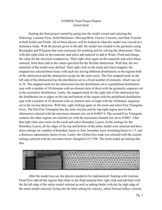
materials of the model were defined. Then right click on the mesh and select mapped, the
mapped was selected three times with each one having different distributions in the regions both
of the obstruction and the obstruction except for the semi-circle. The first mapped mesh on the
left side of the obstruction has the distribution set to a fixed number of elements, which was set
to 36. The mapped mesh for the obstruction has the distribution set to a predefined distribution
type with a number of 10 elements with an element ratio of three with the geometric sequence set
to the symmetric distribution. Lastly, the mapped mesh for the right side of the obstruction has
the distribution set to edges on the top and bottom of the region with the predefined distribution
type with a number of 25 elements with an element ratio of eight with the Arithmetic sequence
set to the reverse direction. With that, right clicking again on the mesh and select Free Triangular
twice. The first Free Triangular has the semi-circular and the top-right region next to the
obstruction selected with the maximum element size set to 0.0067/4. The second Free Triangular
contains the other regions not selected yet with the maximum element size set to 0.0067. After
that right click once more on the mesh and select Boundary Layers. In the settings for the
Boundary Layers, all the edges of the top and bottom of the entire model were selected and have
these settings set: number of boundary layers to four, boundary layer stretching factor to 1.5, and
a thickness adjustments factor of one. Lastly, the Global Size node was selected with the custom
settings selected with the curvature factor changed to 0.3*100. The mesh ended up looking like
this.
After the model was set, the physics needed to be implemented. Starting with Laminar
Fluid Flow add all the regions that relate to the fluid material then right click and add Inlet with
the far left edge of the entire model selected as well as adding Outlet with the far right edge of
the entire model selected. Going into the Inlet setting for velocity, select Normal inflow velocity

2. Pg. 2
and set to 0.004[m/s]*6*s*(1-s)*vel_param(pseudo_time). The program will note that both
pseudo_time and vel_param has not been established. Then going to global parameter and type
in pseudo_time as a new parameter with the value set to one. Then from there right click on
Global Definitions and select Ramps under the Functions tab, the settings will come up for the
ramp. Change the function name to vel_param so that the program will recognize the name and
have the location set to zero, the slope to one, and the cutoff checked with a value of one set.
Lastly, in the Laminar Flow settings under Advanced Setting the “use pseudo time stepping for
stationary equation form” was checked to help aid in convergences. Next, was changing the
Solid Mechanics and selecting all the regions relating to the obstruction. Then right-click on
Solid Mechanics and select the edge Boundary Load and select all the edges except for the
bottom of the obstruction. Thiswas then set to a pressure of p, which was taken from the Laminar
Flow. Then right-click again on the Solid Mechanics and select Edge Fixed Displacement. The
edges from the bottom of the obstruction were selected for the Fixed Displacement. Next, go to
the Moving Mesh physics and in the settings of the parent node and change the geometry shape
order to 1 and the in the Free Deformation Settings change the mesh smoothing type to
Hyperelastic which will help with the convergences. To allow the moving mesh boundary to
move go to definitions right click and under Component Coupling select Integration. With that,
select the top point of the obstruction to allow movement to be shown in the results. To confirm
if the prescribed displacements were in the right direction, the view node under definitions was
selected and the show edge direction arrows were checked. From there the arrows that were
shown should be in the correct direction then create a free deformation and selecting the four
domains around the obstruction. From there right-click on Moving Mesh and select Prescribed
Mesh Displacement for boundaries. That step was done four times and the edges selected with
the correct values matches that shown in the pdf. Then going into the Electric Currents, right-
click and select Electric Potential for boundaries, the bottom edge of the obstruction was selected
and the Electric Potential was set with the value 3.0[V]*volt_param(pseudo_time). Then right-
click again on the Electric Currents and select ground having that set to the top edge of the flow
channel. To make sure this works, going back into Global Definitions and select ramp under the
Function tab from there the location was set to one, the slope to one, and the cutoff checked with
a value of one set. The last physics to be changed was the Heat Transfer in Solids in which the
entire model was selected. From there right click on the node and add in Heat Transfer in Fluids,
Heat Source, Boundary Temperature, and Boundary Outflow. The Heat Transfer in Fluids has all
the domains except for the domains on the obstruction selected. The Heat Source was applied
only to the domains on the obstruction with the general source set to a Total power dissipation
density (ec). The Boundary Temperature was set to 274[K] with the far left edge of the model
selected and the Boundary Outflow has the far right edge of the model selected. With that, all of
the physics have been defined.
Going to the Study node, five steps were then added into the system, which includes the
following: Laminar Flow Only; Laminar Flow, Solid Mechanics, and Moving Mesh; Electric
Currents Only; Electric Currents and Heat Transfer; and All Physics. All of the physics has its

3. Pg. 3
own settings that deal with the pseudo_time as well as any Multiphysics that correlate with the
different steps. The Mesh, Physics, and the Study Steps were altered multiple times in order to
have Comsol to compile and get results close to what was expected. Once Comsol did compile,
the following graphs were created from the data gathered.
Velocity of fluid with Mesh
Total Displacement with Velocity Magnitude showing Obstruction Deformation

4. Pg. 4
Temperature of Fluid with Streamlines
The temperature was not as hot as it should be. The physics from heat source coming off from
the obstruction could be the cause of such a low value that relates to the Electric Potential from
the object, which could be the main issue.
Volumetric Loss Density

5. Pg. 5
Stress occurring on the Obstruction with velocity flow detailing the temperature of the fluid.
The Temperature of the fluid was low which was more than likely caused by the physics from
heat source coming off from the obstruction could be the cause of such a low value which relates
to the Electric Potential from the object which could be the main problem.
Electric potential through the obstruction with amount of current density through the system

6. Pg. 6
Pressure on the Surface
Line graph of the Pressure Distribution on the Obstruction at different pseudo times
The pressures should have a lower value than what was shown in the pdf. This could possibly be
the mesh not being refined enough.

7. Pg. 7
Fluid Velocity occurring between the top of the obstruction and the top of the channel
Three tables were also created to determine the max, min, and average values of velocity and
temperature in the entire x = 0.1 m. All of the graphs that were compiled relied on five data sets.
This done to make what the graphs displayed for the model match what was represented in the
pdf.
In conclusion, there were still some issues with the results as some of the graphs do not
match exactly with what was shown in the pdf. This may be because of a coupling not being set
up correctly for the physics or the steps not set up correctly for the study. Another possibility was
that the mesh was not refined enough which could affect the actual results. However, this
program has pushed the limit what was learned in class and what was expected in the real world.