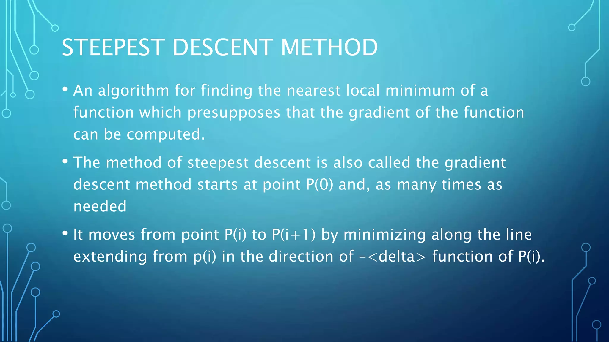
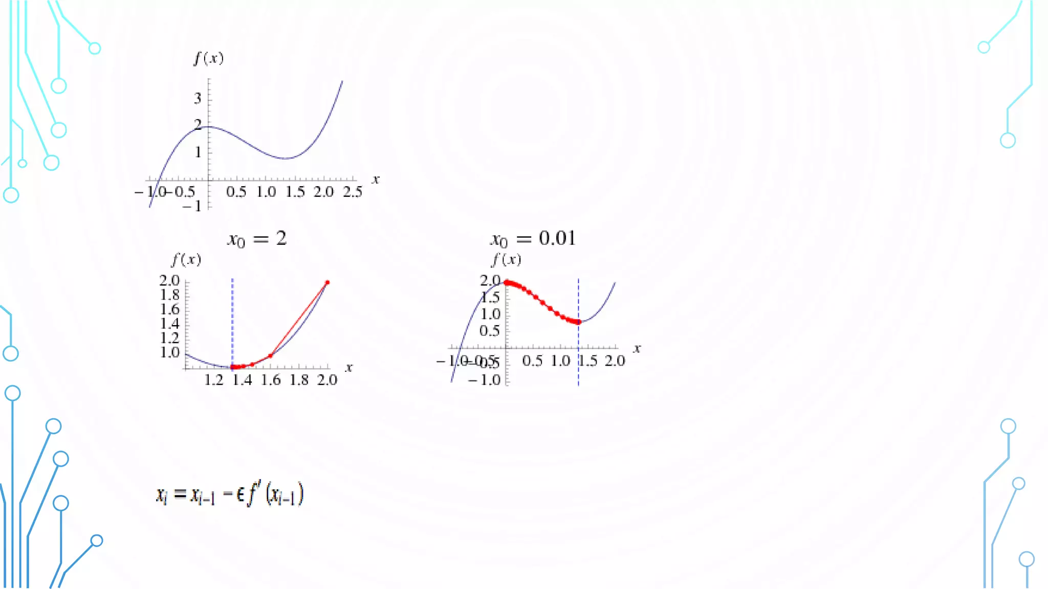
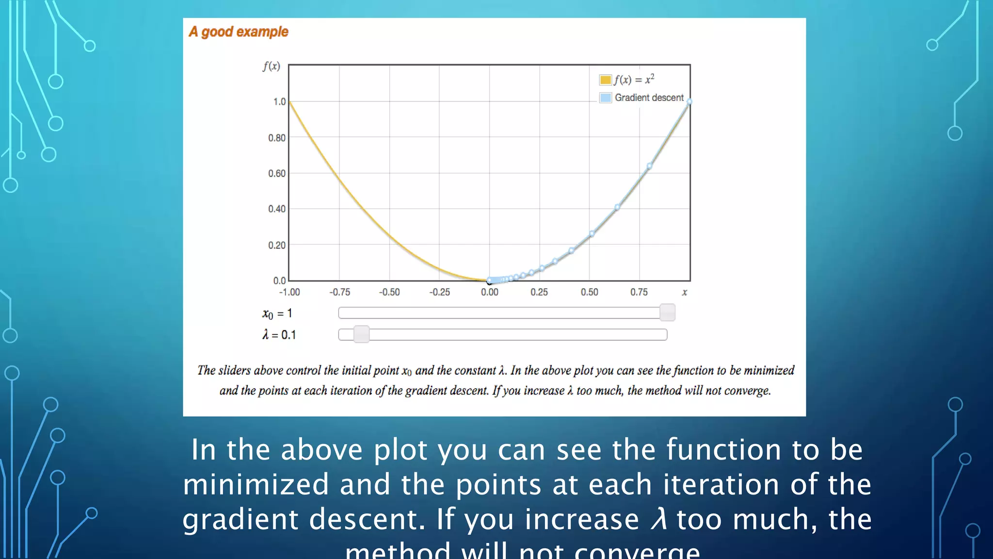
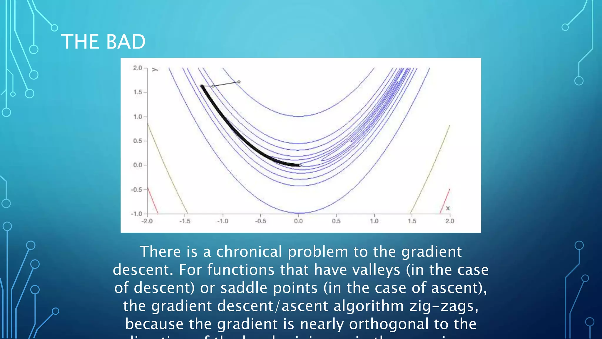
This document discusses the steepest descent method, also called gradient descent, for finding the nearest local minimum of a function. It works by iteratively moving from each point in the direction of the negative gradient to minimize the function. While effective, it can be slow for functions with long, narrow valleys. The step size used in gradient descent is important - too large will diverge it, too small will take a long time to converge. The Lipschitz constant of a function's gradient provides an upper bound for the step size to guarantee convergence.

1. STEEPEST DESCENT METHOD
LESSON 3

2. STEEPEST DESCENT METHOD
• An algorithm for finding the nearest local minimum of a
function which presupposes that the gradient of the function
can be computed.
• The method of steepest descent is also called the gradient
descent method starts at point P(0) and, as many times as
needed
• It moves from point P(i) to P(i+1) by minimizing along the line
extending from p(i) in the direction of –<delta> function of P(i).

4. A DRAWBACK IN THE METHOD
• This method has the severe drawback of requiring a great many
iterations for functions which have long, narrow valley
structures. In such cases, a conjugate gradient method is
preferable.
• To find a local minimum of a function using gradient descent,
one takes steps proportional to the negative of the gradient (or
of the approximate gradient) of the function at the current
point.
• If instead one takes steps proportional to the positive of the
gradient, one approaches a local maximum of that function; the
procedure is then known as gradient ascent

5. A GOOD AND A BAD EXAMPLE

6. In the above plot you can see the function to be
minimized and the points at each iteration of the
gradient descent. If you increase λ too much, the

7. THE BAD
There is a chronical problem to the gradient
descent. For functions that have valleys (in the case
of descent) or saddle points (in the case of ascent),
the gradient descent/ascent algorithm zig-zags,
because the gradient is nearly orthogonal to the

8. THE UGLY
• Imagine the ugliest example you can think of.
• Draw it on your notebook
• Compare it to the guy next to you
• Ugliest example wins

9. ESTIMATING STEP SIZE
• A wrong step size λ may not reach convergence, so a careful
selection of the step size is important.
• Too large it will diverge, too small it will take a long time to converge.
• One option is to choose a fixed step size that will assure convergence
wherever you start gradient descent.
• Another option is to choose a different step size at each iteration
(adaptive step size).

10. MAXIMUM STEP SIZE FOR CONVERGENCE
• Any differentiable function has a maximum derivative value,
i.e., the maximum of the derivatives at all points. If this
maximum is not infinite, this value is known as the Lipschitz
constant and the function is Lipschitz continuous.
‖f(x)−f(y)‖‖x−y‖≤L(f), for any x,y
• This constant is important because it says that, given a certain
function, any derivative will have a smaller value than the
Lipschitz constant.
• The same can be said for the gradient of the function: if the
maximum second derivative is finite, the function is Lipschitz
continuous gradient and that value is the Lipschitz constant of

11. CONTINUED…
‖∇f(x)−∇f(y)‖‖x−y‖≤L(∇f), for any x,y
• For the f(x)=x2 example, the derivative is df(x)/dx=2x and therefore
the function is not Lipschitz continuous.
• But the second derivative is d2f(x)/dx2=2, and the function is Lipschitz
continuous gradient with Lipschitz constant of ∇f=2.

12. CONTINUED …
• Each gradient descent can be viewed as a minimization of the
function:
• xk+1=argminxf(xk)+(x−xk)T∇f(xk)+12λ‖x−xk‖^2
• If we differentiate the equation with respect to x, we get:
• 0=∇f(xk)+1λ(x−xk)
• x=xk−λ∇f(xk)
• It can be shown that for any λ≤1/L(∇f):
• f(x)≤f(xk)+(x−xk)T∇f(xk)+12λ‖x−xk‖^2