SlideShare a Scribd company logo
1 of 49
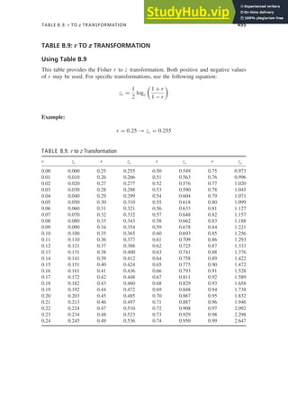
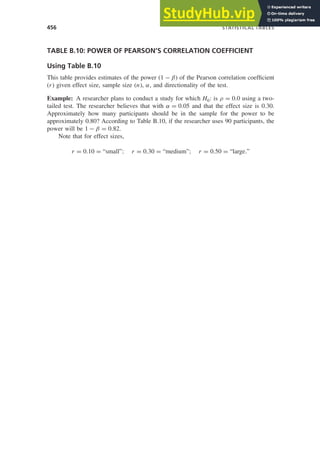
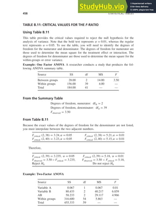
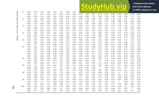
Download to read offline
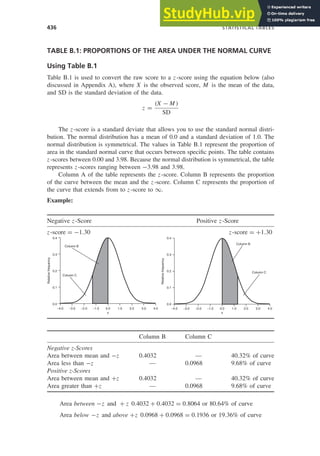
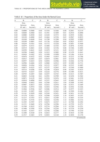
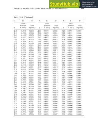
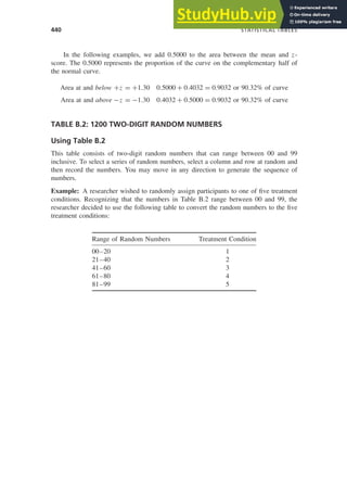
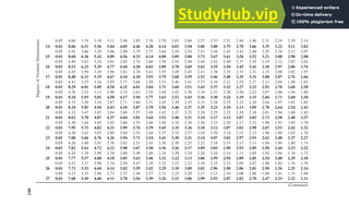
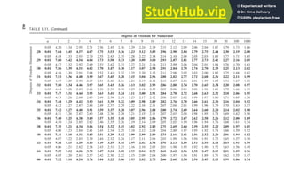
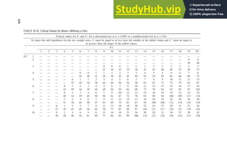
Appendix B
STATISTICAL TABLES
OVERVIEW
Table B.1: Proportions of the Area Under the Normal Curve
Table B.2: 1200 Two-Digit Random Numbers
Table B.3: Critical Values for Student’s t-TEST
Table B.4: Power of Student’s Single Sample t-Ratio
Table B.5: Power of Student’s Two Sample t-Ratio, One-Tailed Tests
Table B.6: Power of Student’s Two Sample t-Ratio, Two-Tailed Tests
Table B.7: Critical Values for Pearson’s Correlation Coefficient
Table B.8 Critical Values for Spearman’s Rank Order Correlation
Coefficient
Table B.9: r to z Transformation
Table B.10: Power of Pearson’s Correlation Coefficient
Table B.11: Critical Values for the F-Ratio
Table B.12: Critical Values for the Fmax Test
Table B.13: Critical Values for the Studentized Range Test
Table B.14: Power of Anova
Table B.15: Critical Values for Chi-Squared
Table B.16: Critical Values for Mann–Whitney u-Test
Understanding Business Research, First Edition. Bart L. Weathington, Christopher J.L. Cunningham,
and David J. Pittenger.
ο›™ 2012 John Wiley & Sons, Inc. Published 2012 by John Wiley & Sons, Inc.
435
436 STATISTICAL TABLES
TABLE B.1: PROPORTIONS OF THE AREA UNDER THE NORMAL CURVE
Using Table B.1
Table B.1 is used to convert the raw score to a z-score using the equation below (also
discussed in Appendix A), where X is the observed score, M is the mean of the data,
and SD is the standard deviation of the data.
z =
(X βˆ’ M )
SD
The z-score is a standard deviate that allows you to use the standard normal distri-
bution. The normal distribution has a mean of 0.0 and a standard deviation of 1.0. The
normal distribution is symmetrical. The values in Table B.1 represent the proportion of
area in the standard normal curve that occurs between specific points. The table contains
z-scores between 0.00 and 3.98. Because the normal distribution is symmetrical, the table
represents z-scores ranging between βˆ’3.98 and 3.98.
Column A of the table represents the z-score. Column B represents the proportion
of the curve between the mean and the z-score. Column C represents the proportion of
the curve that extends from to z-score to ∞.
Example:
Negative z-Score Positive z-Score
z-score = βˆ’1.30 z-score = +1.30
0.0
βˆ’4.0 βˆ’3.0 βˆ’2.0 βˆ’1.0 0.0 1.0 2.0 3.0 4.0
0.1
0.2
Relative
frequency
x
0.3
0.4
Column B
Column C
Relative
frequency
x
0.0
βˆ’4.0 βˆ’3.0 βˆ’2.0 βˆ’1.0 0.0 1.0 2.0 3.0 4.0
0.1
0.2
0.3
0.4
Column B
Column C
Column B Column C
Negative z-Scores
Area between mean and βˆ’z 0.4032 β€” 40.32% of curve
Area less than βˆ’z β€” 0.0968 9.68% of curve
Positive z-Scores
Area between mean and +z 0.4032 β€” 40.32% of curve
Area greater than +z β€” 0.0968 9.68% of curve
Area between βˆ’z and + z 0.4032 + 0.4032 = 0.8064 or 80.64% of curve
Area below βˆ’z and above +z 0.0968 + 0.0968 = 0.1936 or 19.36% of curve
TABLE B.1: PROPORTIONS OF THE AREA UNDER THE NORMAL CURVE 437
TABLE B.1. Proportions of the Area Under the Normal Curve
A B C A B C A B C
Area Area Area
between Area between Area between Area
z M and z beyond z z M and z beyond z z M and z beyond z
0.00 0.0000 0.5000 0.40 0.1554 0.3446 0.80 0.2881 0.2119
0.01 0.0040 0.4960 0.41 0.1591 0.3409 0.81 0.2910 0.2090
0.02 0.0080 0.4920 0.42 0.1628 0.3372 0.82 0.2939 0.2061
0.03 0.0120 0.4880 0.43 0.1664 0.3336 0.83 0.2967 0.2033
0.04 0.0160 0.4840 0.44 0.1700 0.3300 0.84 0.2995 0.2005
0.05 0.0199 0.4801 0.45 0.1736 0.3264 0.85 0.3023 0.1977
0.06 0.0239 0.4761 0.46 0.1772 0.3228 0.86 0.3051 0.1949
0.07 0.0279 0.4721 0.47 0.1808 0.3192 0.87 0.3078 0.1922
0.08 0.0319 0.4681 0.48 0.1844 0.3156 0.88 0.3106 0.1894
0.09 0.0359 0.4641 0.49 0.1879 0.3121 0.89 0.3133 0.1867
0.10 0.0398 0.4602 0.50 0.1915 0.3085 0.90 0.3159 0.1841
0.11 0.0438 0.4562 0.51 0.1950 0.3050 0.91 0.3186 0.1814
0.12 0.0478 0.4522 0.52 0.1985 0.3015 0.92 0.3212 0.1788
0.13 0.0517 0.4483 0.53 0.2019 0.2981 0.93 0.3238 0.1762
0.14 0.0557 0.4443 0.54 0.2054 0.2946 0.94 0.3264 0.1736
0.15 0.0596 0.4404 0.55 0.2088 0.2912 0.95 0.3289 0.1711
0.16 0.0636 0.4364 0.56 0.2123 0.2877 0.96 0.3315 0.1685
0.17 0.0675 0.4325 0.57 0.2157 0.2843 0.97 0.3340 0.1660
0.18 0.0714 0.4286 0.58 0.2190 0.2810 0.98 0.3365 0.1635
0.19 0.0753 0.4247 0.59 0.2224 0.2776 0.99 0.3389 0.1611
0.20 0.0793 0.4207 0.60 0.2257 0.2743 0.99 0.3413 0.1587
0.21 0.0832 0.4168 0.61 0.2291 0.2709 1.01 0.3438 0.1562
0.22 0.0871 0.4129 0.62 0.2324 0.2676 1.02 0.3461 0.1539
0.23 0.0910 0.4090 0.63 0.2357 0.2643 1.03 0.3485 0.1515
0.24 0.0948 0.4052 0.64 0.2389 0.2611 1.04 0.3508 0.1492
0.25 0.0987 0.4013 0.65 0.2422 0.2578 1.05 0.3531 0.1469
0.26 0.1026 0.3974 0.66 0.2454 0.2546 1.06 0.3554 0.1446
0.27 0.1064 0.3936 0.67 0.2486 0.2514 1.07 0.3577 0.1423
0.28 0.1103 0.3897 0.68 0.2517 0.2483 1.08 0.3599 0.1401
0.29 0.1141 0.3859 0.69 0.2549 0.2451 1.09 0.3621 0.1379
0.30 0.1179 0.3821 0.70 0.2580 0.2420 1.10 0.3643 0.1357
0.31 0.1217 0.3783 0.71 0.2611 0.2389 1.11 0.3665 0.1335
0.32 0.1255 0.3745 0.72 0.2642 0.2358 1.12 0.3686 0.1314
0.33 0.1293 0.3707 0.73 0.2673 0.2327 1.13 0.3708 0.1292
0.34 0.1331 0.3669 0.74 0.2704 0.2296 1.14 0.3729 0.1271
0.35 0.1368 0.3632 0.75 0.2734 0.2266 1.15 0.3749 0.1251
0.36 0.1406 0.3594 0.76 0.2764 0.2236 1.16 0.3770 0.1230
0.37 0.1443 0.3557 0.77 0.2794 0.2206 1.17 0.3790 0.1210
0.38 0.1480 0.3520 0.78 0.2823 0.2177 1.18 0.3810 0.1190
0.39 0.1517 0.3483 0.79 0.2852 0.2148 1.19 0.3830 0.1170
(Continued)
438 STATISTICAL TABLES
TABLE B.1. (Continued)
A B C A B C A B C
Area Area Area
between Area between Area between Area
z M and z beyond z z M and z beyond z z M and z beyond z
1.20 0.3849 0.1151 1.60 0.4452 0.0548 2.00 0.4772 0.0228
1.21 0.3869 0.1131 1.61 0.4463 0.0537 2.01 0.4778 0.0222
1.22 0.3888 0.1112 1.62 0.4474 0.0526 2.02 0.4783 0.0217
1.23 0.3907 0.1093 1.63 0.4484 0.0516 2.03 0.4788 0.0212
1.24 0.3925 0.1075 1.64 0.4495 0.0505 2.04 0.4793 0.0207
1.25 0.3944 0.1056 1.65 0.4505 0.0495 2.05 0.4798 0.0202
1.26 0.3962 0.1038 1.66 0.4515 0.0485 2.06 0.4803 0.0197
1.27 0.3980 0.1020 1.67 0.4525 0.0475 2.07 0.4808 0.0192
1.28 0.3997 0.1003 1.68 0.4535 0.0465 2.08 0.4812 0.0188
1.29 0.4015 0.0985 1.69 0.4545 0.0455 2.09 0.4817 0.0183
1.30 0.4032 0.0968 1.70 0.4554 0.0446 2.10 0.4821 0.0179
1.31 0.4049 0.0951 1.71 0.4564 0.0436 2.11 0.4826 0.0174
1.32 0.4066 0.0934 1.72 0.4573 0.0427 2.12 0.4830 0.0170
1.33 0.4082 0.0918 1.73 0.4582 0.0418 2.13 0.4834 0.0166
1.34 0.4099 0.0901 1.74 0.4591 0.0409 2.14 0.4838 0.0162
1.35 0.4115 0.0885 1.75 0.4599 0.0401 2.15 0.4842 0.0158
1.36 0.4131 0.0869 1.76 0.4608 0.0392 2.16 0.4846 0.0154
1.37 0.4147 0.0853 1.77 0.4616 0.0384 2.17 0.4850 0.0150
1.38 0.4162 0.0838 1.78 0.4625 0.0375 2.18 0.4854 0.0146
1.39 0.4177 0.0823 1.79 0.4633 0.0367 2.19 0.4857 0.0143
1.40 0.4192 0.0808 1.80 0.4641 0.0359 2.20 0.4861 0.0139
1.41 0.4207 0.0793 1.81 0.4649 0.0351 2.21 0.4864 0.0136
1.42 0.4222 0.0778 1.82 0.4656 0.0344 2.22 0.4868 0.0132
1.43 0.4236 0.0764 1.83 0.4664 0.0336 2.23 0.4871 0.0129
1.44 0.4251 0.0749 1.84 0.4671 0.0329 2.24 0.4875 0.0125
1.45 0.4265 0.0735 1.85 0.4678 0.0322 2.25 0.4878 0.0122
1.46 0.4279 0.0721 1.86 0.4686 0.0314 2.26 0.4881 0.0119
1.47 0.4292 0.0708 1.87 0.4693 0.0307 2.27 0.4884 0.0116
1.48 0.4306 0.0694 1.88 0.4699 0.0301 2.28 0.4887 0.0113
1.49 0.4319 0.0681 1.89 0.4706 0.0294 2.29 0.4890 0.0110
1.50 0.4332 0.0668 1.90 0.4713 0.0287 2.30 0.4893 0.0107
1.51 0.4345 0.0655 1.91 0.4719 0.0281 2.31 0.4896 0.0104
1.52 0.4357 0.0643 1.92 0.4726 0.0274 2.32 0.4898 0.0102
1.53 0.4370 0.0630 1.93 0.4732 0.0268 2.33 0.4901 0.0099
1.54 0.4382 0.0618 1.94 0.4738 0.0262 2.34 0.4904 0.0096
1.55 0.4394 0.0606 1.95 0.4744 0.0256 2.35 0.4906 0.0094
1.56 0.4406 0.0594 1.96 0.4750 0.0250 2.36 0.4909 0.0091
1.57 0.4418 0.0582 1.97 0.4756 0.0244 2.37 0.4911 0.0089
1.58 0.4429 0.0571 1.98 0.4761 0.0239 2.38 0.4913 0.0087
1.59 0.4441 0.0559 1.99 0.4767 0.0233 2.39 0.4916 0.0084
TABLE B.1: PROPORTIONS OF THE AREA UNDER THE NORMAL CURVE 439
TABLE B.1. (Continued)
A B C A B C A B C
Area Area Area
between Area between Area between Area
z M and z beyond z z M and z beyond z z M and z beyond z
2.40 0.4918 0.0082 2.80 0.4974 0.0026 3.20 0.4993 0.0007
2.41 0.4920 0.0080 2.81 0.4975 0.0025 3.22 0.4994 0.0006
2.42 0.4922 0.0078 2.82 0.4976 0.0024 3.24 0.4994 0.0006
2.43 0.4925 0.0075 2.83 0.4977 0.0023 3.26 0.4994 0.0006
2.44 0.4927 0.0073 2.84 0.4977 0.0023 3.28 0.4995 0.0005
2.45 0.4929 0.0071 2.85 0.4978 0.0022 3.30 0.4995 0.0005
2.46 0.4931 0.0069 2.86 0.4979 0.0021 3.32 0.4995 0.0005
2.47 0.4932 0.0068 2.87 0.4979 0.0021 3.34 0.4996 0.0004
2.48 0.4934 0.0066 2.88 0.4980 0.0020 3.36 0.4996 0.0004
2.49 0.4936 0.0064 2.89 0.4981 0.0019 3.38 0.4996 0.0004
2.50 0.4938 0.0062 2.90 0.4981 0.0019 3.40 0.4997 0.0003
2.51 0.4940 0.0060 2.91 0.4982 0.0018 3.42 0.4997 0.0003
2.52 0.4941 0.0059 2.92 0.4982 0.0018 3.44 0.4997 0.0003
2.53 0.4943 0.0057 2.93 0.4983 0.0017 3.46 0.4997 0.0003
2.54 0.4945 0.0055 2.94 0.4984 0.0016 3.48 0.4997 0.0003
2.55 0.4946 0.0054 2.95 0.4984 0.0016 3.50 0.4998 0.0002
2.56 0.4948 0.0052 2.96 0.4985 0.0015 3.52 0.4998 0.0002
2.57 0.4949 0.0051 2.97 0.4985 0.0015 3.54 0.4998 0.0002
2.58 0.4951 0.0049 2.98 0.4986 0.0014 3.56 0.4998 0.0002
2.59 0.4952 0.0048 2.99 0.4986 0.0014 3.58 0.4998 0.0002
2.60 0.4953 0.0047 3.00 0.4987 0.0013 3.60 0.4998 0.0002
2.61 0.4955 0.0045 3.01 0.4987 0.0013 3.62 0.4999 0.0001
2.62 0.4956 0.0044 3.02 0.4987 0.0013 3.64 0.4999 0.0001
2.63 0.4957 0.0043 3.03 0.4988 0.0012 3.66 0.4999 0.0001
2.64 0.4959 0.0041 3.04 0.4988 0.0012 3.68 0.4999 0.0001
2.65 0.4960 0.0040 3.05 0.4989 0.0011 3.70 0.4999 0.0001
2.66 0.4961 0.0039 3.06 0.4989 0.0011 3.72 0.4999 0.0001
2.67 0.4962 0.0038 3.07 0.4989 0.0011 3.74 0.4999 0.0001
2.68 0.4963 0.0037 3.08 0.4990 0.0010 3.76 0.4999 0.0001
2.69 0.4964 0.0036 3.09 0.4990 0.0010 3.78 0.4999 0.0001
2.70 0.4965 0.0035 3.10 0.4990 0.0010 3.80 0.4999 0.0001
2.71 0.4966 0.0034 3.11 0.4991 0.0009 3.82 0.4999 0.0001
2.72 0.4967 0.0033 3.12 0.4991 0.0009 3.84 0.4999 0.0001
2.73 0.4968 0.0032 3.13 0.4991 0.0009 3.86 0.4999 0.0001
2.74 0.4969 0.0031 3.14 0.4992 0.0008 3.88 0.4999 0.0001
2.75 0.4970 0.0030 3.15 0.4992 0.0008 3.90 0.5000 0.0000
2.76 0.4971 0.0029 3.16 0.4992 0.0008 3.92 0.5000 0.0000
2.77 0.4972 0.0028 3.17 0.4992 0.0008 3.94 0.5000 0.0000
2.78 0.4973 0.0027 3.18 0.4993 0.0007 3.96 0.5000 0.0000
2.79 0.4974 0.0026 3.19 0.4993 0.0007 3.98 0.5000 0.0000
440 STATISTICAL TABLES
In the following examples, we add 0.5000 to the area between the mean and z-
score. The 0.5000 represents the proportion of the curve on the complementary half of
the normal curve.
Area at and below +z = +1.30 0.5000 + 0.4032 = 0.9032 or 90.32% of curve
Area at and above βˆ’z = βˆ’1.30 0.4032 + 0.5000 = 0.9032 or 90.32% of curve
TABLE B.2: 1200 TWO-DIGIT RANDOM NUMBERS
Using Table B.2
This table consists of two-digit random numbers that can range between 00 and 99
inclusive. To select a series of random numbers, select a column and row at random and
then record the numbers. You may move in any direction to generate the sequence of
numbers.
Example: A researcher wished to randomly assign participants to one of five treatment
conditions. Recognizing that the numbers in Table B.2 range between 00 and 99, the
researcher decided to use the following table to convert the random numbers to the five
treatment conditions:
Range of Random Numbers Treatment Condition
00–20 1
21–40 2
41–60 3
61–80 4
81–99 5
TABLE B.2. 1200 Two-Digit Random Numbers
1 2 3 4 5 6 7 8 9 10 11 12 13 14 15 16 17 18 19 20 21 22 23 24
1 43 41 16 31 22 44 10 41 45 00 47 19 43 67 83 02 79 05 98 92 64 82 06 89
2 26 44 01 04 28 85 11 91 23 02 39 79 44 45 93 20 17 91 35 15 25 82 18 41
3 83 39 26 84 04 16 89 79 68 85 61 63 03 20 17 76 95 80 27 39 35 82 10 86
4 65 94 48 27 77 65 34 95 04 51 78 90 14 76 90 83 17 76 69 50 34 01 25 08
5 89 38 32 05 09 49 87 93 21 24 88 74 30 94 26 19 23 72 94 80 90 24 55 44
6 77 80 30 43 26 01 43 46 66 40 52 00 44 69 84 10 48 96 49 85 49 84 97 41
7 43 42 26 74 51 05 56 43 06 80 58 22 57 02 11 95 00 91 88 17 71 98 32 56
8 76 76 61 17 69 06 73 37 77 06 36 28 05 73 31 04 44 33 40 74 46 26 02 99
9 42 05 88 83 15 05 28 52 88 78 88 66 50 80 24 38 31 20 48 73 18 85 18 90
10 46 74 76 34 97 40 59 34 86 11 50 98 69 59 46 74 59 60 98 76 96 42 34 83
11 67 15 82 94 59 55 27 99 02 34 47 34 88 98 72 15 38 73 57 42 56 09 85 83
12 03 58 51 69 14 89 24 06 35 31 16 65 71 76 04 80 01 36 00 67 78 73 07 37
13 79 98 19 32 25 95 89 54 20 78 29 81 96 34 62 53 26 09 02 04 63 95 03 53
14 56 12 61 36 21 69 96 06 22 06 01 80 57 72 23 55 05 74 42 55 91 45 60 91
15 58 80 33 35 75 33 35 42 06 79 73 29 89 73 99 07 05 54 42 77 78 99 33 92
16 31 51 77 53 92 51 35 71 34 46 79 43 76 15 76 46 40 04 36 84 83 64 56 73
17 25 77 95 61 71 10 82 51 57 88 29 59 55 84 71 89 64 34 38 33 11 45 47 19
18 02 12 81 84 23 80 58 65 74 13 46 09 33 66 86 74 94 96 07 22 52 39 31 36
19 18 38 40 30 34 27 70 62 35 71 48 96 73 74 28 61 15 37 23 16 91 29 03 06
20 31 76 47 77 59 14 66 85 27 10 63 58 48 66 66 17 91 16 55 70 30 53 05 94
21 50 93 33 61 20 55 10 61 08 76 62 14 22 65 44 95 75 68 94 76 51 21 22 12
22 45 75 89 11 64 06 22 39 20 04 91 47 16 48 19 93 12 02 17 15 94 74 77 37
23 17 97 59 42 77 26 29 88 66 62 53 28 95 01 10 85 31 10 25 75 10 35 99 60
24 23 25 86 94 12 75 66 93 87 95 09 48 85 43 20 94 00 38 53 45 11 77 01 66
(Continued)
441
TABLE B.2. (Continued)
1 2 3 4 5 6 7 8 9 10 11 12 13 14 15 16 17 18 19 20 21 22 23 24
25 63 17 05 28 67 39 72 85 02 34 69 56 53 66 09 38 72 31 85 29 62 18 29 37
26 99 81 28 63 05 26 66 16 66 69 18 56 26 53 29 38 08 04 27 93 54 83 53 15
27 86 72 54 89 57 45 05 82 32 64 93 24 83 44 56 65 29 68 69 14 70 79 92 39
28 42 50 86 19 08 81 57 09 69 35 29 06 52 43 53 99 57 55 30 63 63 67 94 94
29 42 80 75 06 05 62 69 04 90 49 10 48 34 21 63 94 19 99 96 79 83 41 86 38
30 82 48 69 65 59 74 64 25 66 93 32 56 14 57 80 10 36 17 39 48 46 94 88 43
31 24 81 98 33 40 89 60 97 28 64 78 93 07 84 07 02 63 35 64 30 29 49 37 00
32 15 84 59 73 01 21 67 43 43 74 00 28 64 66 03 80 60 08 51 67 51 89 00 46
33 92 31 60 34 23 72 00 19 78 73 80 36 51 54 45 76 17 34 35 74 78 20 49 95
34 05 80 10 40 30 63 25 78 91 13 77 39 90 78 89 17 45 76 28 64 12 37 60 34
35 67 51 92 66 84 33 15 34 42 73 54 93 02 01 19 87 36 58 08 11 58 38 88 98
36 71 44 83 33 92 84 96 76 87 24 59 41 71 36 86 14 54 31 41 25 15 59 74 52
37 43 13 62 58 75 90 94 10 65 16 51 90 01 40 18 21 51 82 69 91 65 91 22 32
38 97 55 94 52 18 65 73 90 55 80 51 05 60 53 01 52 46 57 21 05 76 61 05 23
39 32 75 70 24 04 98 03 79 84 34 50 06 25 00 05 00 04 25 68 58 99 48 06 80
40 23 87 76 65 51 19 93 54 81 09 71 83 97 24 90 01 81 14 70 16 07 16 05 93
41 21 77 33 17 02 64 55 23 21 84 80 02 79 30 61 46 33 94 28 92 44 27 76 20
42 90 11 17 05 24 52 08 39 94 07 43 58 33 72 04 51 81 79 63 70 94 71 71 68
43 89 00 39 09 55 13 96 24 47 81 18 37 82 37 37 01 95 82 38 57 20 20 35 83
44 58 65 18 34 73 85 20 47 04 68 77 28 80 14 37 24 97 62 87 38 09 09 08 50
45 80 35 64 10 03 18 24 41 54 12 99 97 50 14 15 80 71 87 47 79 50 62 87 42
46 87 26 52 18 56 47 76 29 40 08 12 07 40 49 29 70 60 74 20 50 51 00 17 42
47 54 23 81 36 70 93 10 05 39 54 20 49 10 70 49 13 37 59 44 52 98 13 64 48
48 72 08 17 30 70 44 08 10 25 81 53 39 81 67 13 80 74 09 71 06 95 05 17 00
49 34 59 02 12 20 31 15 96 18 12 37 32 25 96 71 52 78 01 77 18 63 66 96 09
50 97 89 00 94 82 17 49 92 29 73 30 17 78 53 45 29 39 24 95 61 63 76 90 86
442
TABLE B.3: CRITICAL VALUES FOR STUDENT’S t-TEST 443
TABLE B.3: CRITICAL VALUES FOR STUDENT’S t-TEST
Using Table B.3
For any given df, the table shows the values of tcritical corresponding to various levels of
probability. The tobserved is statistically significant at a given level when it is equal to or
greater than the value shown in the table.
For the single sample t-ratio, df = N βˆ’ 1.
For the two sample t-ratio, df = (n1 βˆ’ 1) + (n2 βˆ’ 1).
Examples:
Nondirectional Hypothesis
H0: ΞΌ βˆ’ ΞΌ = 0 H1: ΞΌ βˆ’ ΞΌ = 0 Ξ± = 0.05, df = 30
tcritical = Β±2.042 If |tobserved| β‰₯ |tcritical| then reject H0
Directional Hypothesis
H0: ΞΌ βˆ’ ΞΌ ≀ 0 H1: ΞΌ βˆ’ ΞΌ  0 Ξ± = 0.05, df = 30
tcritical = +1.697 If tobserved β‰₯ tcritical then reject H0
H0: ΞΌ βˆ’ ΞΌ β‰₯ 0 H1: ΞΌ βˆ’ ΞΌ  0 Ξ± = 0.05, df = 30
tcritical = βˆ’1.697 If tobserved ≀ tcritical then reject H0
444 STATISTICAL TABLES
TABLE B.3. Critical Values for Student’s t-TEST
Level of Significance of a One-Tailed or Directional Test
H0: ΞΌ βˆ’ ΞΌ β‰₯ 0 or H0: ΞΌ βˆ’ ΞΌ ≀ 0
Ξ± = 0.10 Ξ± = 0.05 Ξ± = .025 Ξ± = 0.01 Ξ± = 0.005 Ξ± = 0.0005
1 βˆ’ Ξ± = 0.90 1 βˆ’ Ξ± = 0.95 1 βˆ’ Ξ± = 0.975 1 βˆ’ Ξ± = 0.99 1 βˆ’ Ξ± = 0.995 1 βˆ’ Ξ± = 0.9995
Level of Significance of a Two-Tailed or Nondirectional Test
H0: ΞΌ βˆ’ ΞΌ = 0
Ξ± = 0.20 Ξ± = 0.10 Ξ± = 0.05 Ξ± = 0.02 Ξ± = 0.01 Ξ± = 0.001
df 1 βˆ’ Ξ± = 0.80 1 βˆ’ Ξ± = 0.90 1 βˆ’ Ξ± = 0.95 1 βˆ’ Ξ± = 0.98 1 βˆ’ Ξ± = 0.99 1 βˆ’ Ξ± = 0.999
1 3.078 6.314 12.706 31.821 63.656 636.578
2 1.886 2.920 4.303 6.965 9.925 31.600
3 1.638 2.353 3.182 4.541 5.841 12.924
4 1.533 2.132 2.776 3.747 4.604 8.610
5 1.476 2.015 2.571 3.365 4.032 6.869
6 1.440 1.943 2.447 3.143 3.707 5.959
7 1.415 1.895 2.365 2.998 3.499 5.408
8 1.397 1.860 2.306 2.896 3.355 5.041
9 1.383 1.833 2.262 2.821 3.250 4.781
10 1.372 1.812 2.228 2.764 3.169 4.587
11 1.363 1.796 2.201 2.718 3.106 4.437
12 1.356 1.782 2.179 2.681 3.055 4.318
13 1.350 1.771 2.160 2.650 3.012 4.221
14 1.345 1.761 2.145 2.624 2.977 4.140
15 1.341 1.753 2.131 2.602 2.947 4.073
16 1.337 1.746 2.120 2.583 2.921 4.015
17 1.333 1.740 2.110 2.567 2.898 3.965
18 1.330 1.734 2.101 2.552 2.878 3.922
19 1.328 1.729 2.093 2.539 2.861 3.883
20 1.325 1.725 2.086 2.528 2.845 3.850
21 1.323 1.721 2.080 2.518 2.831 3.819
22 1.321 1.717 2.074 2.508 2.819 3.792
23 1.319 1.714 2.069 2.500 2.807 3.768
24 1.318 1.711 2.064 2.492 2.797 3.745
25 1.316 1.708 2.060 2.485 2.787 3.725
26 1.315 1.706 2.056 2.479 2.779 3.707
27 1.314 1.703 2.052 2.473 2.771 3.689
28 1.313 1.701 2.048 2.467 2.763 3.674
29 1.311 1.699 2.045 2.462 2.756 3.660
30 1.310 1.697 2.042 2.457 2.750 3.646
40 1.303 1.684 2.021 2.423 2.704 3.551
50 1.299 1.676 2.009 2.403 2.678 3.496
60 1.296 1.671 2.000 2.390 2.660 3.460
70 1.294 1.667 1.994 2.381 2.648 3.435
80 1.292 1.664 1.990 2.374 2.639 3.416
90 1.291 1.662 1.987 2.368 2.632 3.402
100 1.290 1.660 1.984 2.364 2.626 3.390
150 1.287 1.655 1.976 2.351 2.609 3.357
200 1.286 1.653 1.972 2.345 2.601 3.340
500 1.283 1.648 1.965 2.334 2.586 3.310
1000 1.282 1.646 1.962 2.330 2.581 3.300
∞ 1.282 1.645 1.960 2.326 2.576 3.290
TABLE B.4: POWER OF STUDENT’S SINGLE SAMPLE t-RATIO 445
TABLE B.4: POWER OF STUDENT’S SINGLE SAMPLE t-RATIO
Using Table B.4
This table provides the power (1 βˆ’ Ξ²) of the single sample t-ratio given effect size,
sample size (n), Ξ±, and directionality of the test.
Example: A researcher plans to conduct a study for which H0: is ΞΌ = 12.0 using a
two-tailed t-ratio. The researcher believes that with Ξ± = 0.05 and that the effect size is
0.20. Approximately how many participants should be in the sample for the power to be
approximately 0.80? According to Table B.4, if the researcher uses 200 participants, the
power will be 1 βˆ’ Ξ² = 0.83.
Note that for Cohen’s d, an estimate of effect size is as follows:
d = 0.20 = β€œsmall”; d = 0.50 = β€œmedium”; d = 0.80 = β€œlarge.”
446 STATISTICAL TABLES
TABLE B.4. Power of Student’s Single Sample t-Ratio
Power Table: Single Sample t-Ratio
Ξ± = 0.05 Two-Tailed Ξ± = 0.01 Two-Tailed
n tc 0.10 0.20 0.50 0.80 tc 0.10 0.20 0.50 0.80
5 2.306 0.07 0.09 0.19 0.37 3.355 0.02 0.03 0.07 0.16
6 2.228 0.07 0.09 0.22 0.44 3.169 0.02 0.03 0.08 0.21
7 2.179 0.07 0.09 0.24 0.50 3.055 0.02 0.03 0.10 0.25
8 2.145 0.07 0.10 0.27 0.57 2.977 0.02 0.03 0.11 0.30
9 2.120 0.07 0.10 0.30 0.62 2.921 0.02 0.03 0.13 0.35
10 2.101 0.07 0.10 0.33 0.67 2.878 0.02 0.03 0.14 0.40
11 2.086 0.07 0.11 0.35 0.72 2.845 0.02 0.03 0.16 0.45
12 2.074 0.07 0.11 0.38 0.76 2.819 0.02 0.03 0.18 0.50
13 2.064 0.07 0.11 0.41 0.80 2.797 0.02 0.04 0.19 0.54
14 2.056 0.07 0.12 0.44 0.83 2.779 0.02 0.04 0.21 0.59
15 2.048 0.07 0.12 0.46 0.86 2.763 0.02 0.04 0.23 0.63
16 2.042 0.07 0.12 0.49 0.88 2.750 0.02 0.04 0.25 0.67
17 2.037 0.07 0.13 0.51 0.90 2.738 0.02 0.04 0.27 0.71
18 2.032 0.07 0.13 0.54 0.92 2.728 0.02 0.04 0.29 0.74
19 2.028 0.07 0.14 0.56 0.94 2.719 0.02 0.05 0.31 0.78
20 2.024 0.08 0.14 0.59 0.95 2.712 0.02 0.05 0.33 0.80
21 2.021 0.08 0.14 0.61 0.96 2.704 0.02 0.05 0.35 0.83
22 2.018 0.08 0.15 0.63 0.97 2.698 0.02 0.05 0.37 0.85
23 2.015 0.08 0.15 0.65 0.97 2.692 0.02 0.05 0.39 0.87
24 2.013 0.08 0.16 0.67 0.98 2.687 0.02 0.05 0.41 0.89
25 2.011 0.08 0.16 0.69 0.98 2.682 0.02 0.06 0.43 0.91
30 2.002 0.08 0.18 0.78 0.99 2.663 0.02 0.07 0.53 0.96
40 1.991 0.09 0.23 0.89 0.99 2.640 0.03 0.09 0.70 0.99
50 1.984 0.10 0.28 0.95 0.99 2.627 0.03 0.11 0.82 0.99
60 1.980 0.11 0.32 0.98 0.99 2.618 0.04 0.14 0.90 0.99
70 1.977 0.13 0.37 0.99 0.99 2.612 0.04 0.17 0.95 0.99
80 1.975 0.14 0.42 0.99 0.99 2.607 0.04 0.20 0.98 0.99
90 1.973 0.15 0.46 0.99 0.99 2.604 0.05 0.23 0.99 0.99
100 1.972 0.16 0.50 0.99 0.99 2.601 0.05 0.26 0.99 0.99
150 1.968 0.22 0.69 0.99 0.99 2.592 0.08 0.43 0.99 0.99
200 1.966 0.28 0.82 0.99 0.99 2.588 0.11 0.59 0.99 0.99
250 1.965 0.34 0.90 0.99 0.99 2.586 0.15 0.72 0.99 0.99
300 1.964 0.39 0.95 0.99 0.99 2.584 0.18 0.82 0.99 0.99
350 1.963 0.45 0.98 0.99 0.99 2.583 0.22 0.89 0.99 0.99
400 1.963 0.51 0.99 0.99 0.99 2.582 0.26 0.94 0.99 0.99
500 1.962 0.61 0.99 0.99 0.99 2.581 0.35 0.98 0.99 0.99
600 1.962 0.69 0.99 0.99 0.99 2.580 0.43 0.99 0.99 0.99
700 1.962 0.76 0.99 0.99 0.99 2.579 0.51 0.99 0.99 0.99
800 1.961 0.82 0.99 0.99 0.99 2.579 0.59 0.99 0.99 0.99
900 1.961 0.87 0.99 0.99 0.99 2.579 0.66 0.99 0.99 0.99
1000 1.961 0.90 0.99 0.99 0.99 2.578 0.72 0.99 0.99 0.99
TABLE B.5: POWER OF STUDENT’S TWO SAMPLE t-RATIO, ONE-TAILED TESTS 447
TABLE B.5: POWER OF STUDENT’S TWO SAMPLE t-RATIO, ONE-TAILED
TESTS
0.4
Reject null
Ξ±
0.3
0.2
Relative
frequency
0.1
0.0
βˆ’3 βˆ’2 βˆ’1 0
t
1
Fail to reject null
2 3
Reject null
Ξ±
Fail to reject null
0.4
0.3
0.2
Relative
frequency
0.1
0.0
βˆ’3 βˆ’1
βˆ’2
t
1
0 2 3
Using Table B.5
This table provides the power (1 βˆ’ Ξ²) of the two sample t-ratio given effect size, sample
size (n), and Ξ± when the researcher uses a directional test.
Example: A researcher plans to conduct a study for which H0: is ΞΌ1 ≀ ΞΌ2 using a
one-tailed t-ratio. The researcher believes that with Ξ± = 0.05 and that the effect size is
0.20. Approximately how many participants should be in the sample for power to be
approximately 0.80? According to Table B.5, if the researcher uses 300 participants in
each sample, the power will be 1 βˆ’ Ξ² = 0.81.
Note that for Cohen’s d, an estimate of effect size:
d = 0.20 = β€œsmall”; d = 0.50 = β€œmedium”; d = 0.80 = β€œlarge.”
448 STATISTICAL TABLES
TABLE B.5. Power of Student’s Two Sample t-Ratio, One-Tailed Tests
Power Table: Two Sample t-Ratio, One-Tailed Tests
Ξ± = 0.05 One-Tailed Ξ± = 0.01 One-Tailed
n tc 0.10 0.20 0.50 0.80 tc 0.10 0.20 0.50 0.80
5 1.860 0.12 0.13 0.21 0.33 2.896 0.04 0.04 0.07 0.13
6 1.812 0.12 0.14 0.22 0.38 2.764 0.03 0.04 0.08 0.15
7 1.782 0.12 0.14 0.24 0.42 2.681 0.03 0.04 0.08 0.18
8 1.761 0.12 0.14 0.26 0.46 2.624 0.03 0.04 0.09 0.21
9 1.746 0.12 0.14 0.28 0.50 2.583 0.03 0.04 0.10 0.23
10 1.734 0.12 0.14 0.29 0.54 2.552 0.03 0.04 0.11 0.26
11 1.725 0.12 0.14 0.31 0.57 2.528 0.03 0.04 0.12 0.29
12 1.717 0.12 0.15 0.33 0.61 2.508 0.03 0.04 0.13 0.32
13 1.711 0.12 0.15 0.35 0.64 2.492 0.03 0.04 0.14 0.35
14 1.706 0.12 0.15 0.36 0.67 2.479 0.03 0.04 0.15 0.37
15 1.701 0.12 0.15 0.38 0.70 2.467 0.03 0.04 0.16 0.40
16 1.697 0.12 0.16 0.40 0.73 2.457 0.03 0.04 0.17 0.43
17 1.694 0.12 0.16 0.41 0.75 2.449 0.03 0.05 0.18 0.46
18 1.691 0.12 0.16 0.43 0.78 2.441 0.03 0.05 0.19 0.49
19 1.688 0.12 0.16 0.45 0.80 2.434 0.03 0.05 0.20 0.52
20 1.686 0.12 0.17 0.46 0.82 2.429 0.03 0.05 0.21 0.54
21 1.684 0.12 0.17 0.48 0.84 2.423 0.03 0.05 0.22 0.57
22 1.682 0.12 0.17 0.50 0.85 2.418 0.03 0.05 0.23 0.59
23 1.680 0.12 0.17 0.51 0.87 2.414 0.03 0.05 0.24 0.62
24 1.679 0.12 0.18 0.53 0.88 2.410 0.03 0.05 0.25 0.64
25 1.677 0.12 0.18 0.54 0.89 2.407 0.03 0.05 0.26 0.66
30 1.672 0.13 0.19 0.61 0.94 2.392 0.03 0.06 0.32 0.76
40 1.665 0.13 0.22 0.73 0.98 2.375 0.03 0.07 0.44 0.89
50 1.661 0.14 0.25 0.82 0.99 2.365 0.04 0.09 0.55 0.96
60 1.658 0.15 0.28 0.88 0.99 2.358 0.04 0.10 0.65 0.99
70 1.656 0.15 0.31 0.92 0.99 2.354 0.04 0.12 0.73 0.99
80 1.655 0.16 0.34 0.95 0.99 2.350 0.04 0.13 0.80 0.99
90 1.653 0.17 0.37 0.97 0.99 2.347 0.05 0.15 0.85 0.99
100 1.653 0.18 0.40 0.98 0.99 2.345 0.05 0.17 0.90 0.99
150 1.650 0.21 0.53 0.99 0.99 2.339 0.07 0.26 0.99 0.99
200 1.649 0.25 0.64 0.99 0.99 2.336 0.09 0.35 0.99 0.99
250 1.648 0.29 0.74 0.99 0.99 2.334 0.10 0.45 0.99 0.99
300 1.647 0.33 0.81 0.99 0.99 2.333 0.12 0.54 0.99 0.99
350 1.647 0.36 0.86 0.99 0.99 2.332 0.14 0.62 0.99 0.99
400 1.647 0.40 0.90 0.99 0.99 2.331 0.17 0.69 0.99 0.99
500 1.646 0.47 0.96 0.99 0.99 2.330 0.21 0.81 0.99 0.99
600 1.646 0.53 0.98 0.99 0.99 2.329 0.26 0.89 0.99 0.99
700 1.646 0.59 0.99 0.99 0.99 2.329 0.30 0.94 0.99 0.99
800 1.646 0.64 0.99 0.99 0.99 2.329 0.35 0.97 0.99 0.99
900 1.646 0.69 0.99 0.99 0.99 2.328 0.40 0.98 0.99 0.99
1000 1.646 0.74 0.99 0.99 0.99 2.328 0.45 0.99 0.99 0.99
TABLE B.6: POWER OF STUDENT’S TWO SAMPLE t-RATIO, TWO-TAILED TESTS 449
TABLE B.6: POWER OF STUDENT’S TWO SAMPLE t-RATIO,
TWO-TAILED TESTS
0.4
Reject null
a/2
Reject null
a/2
0.3
0.2
Relative
frequency
0.1
0.0
βˆ’3 βˆ’2 βˆ’1 0
t
1
Fail to reject null
2 3
Using Table B.6
This table provides the power (1 βˆ’ Ξ²) of the two sample t-ratio given effect size, sample
size (n), and Ξ± when the researcher uses a nondirectional test.
Example: A researcher plans to conduct a study for which H0: is ΞΌ1 = ΞΌ2 using a
two-tailed t-ratio. The researcher believes that with Ξ± = 0.05 and that the effect size is
0.20. Approximately how many participants should be in the sample for the power to be
approximately 0.80? According to Table B.6, if the researcher uses 400 participants in
each group, the power will be 1 βˆ’ Ξ² = 0.82.
Note that for Cohen’s d, an estimate of effect size:
d = 0.20 = β€œsmall”; d = 0.50 = β€œmedium”; d = 0.80 = β€œlarge.”
450 STATISTICAL TABLES
TABLE B.6. Power of Student’s Two Sample t-Ratio, Two-Tailed Tests
Power Table: Two Sample t-Ratio, Two-Tailed Tests
Ξ± = 0.05 Two-Tailed Ξ± = 0.01 Two-Tailed
n tc 0.10 0.20 0.50 0.80 tc 0.10 0.20 0.50 0.80
5 2.306 0.07 0.08 0.13 0.22 3.355 0.02 0.02 0.04 0.08
6 2.228 0.07 0.08 0.14 0.26 3.169 0.02 0.02 0.05 0.10
7 2.179 0.07 0.08 0.15 0.29 3.055 0.02 0.02 0.05 0.12
8 2.145 0.07 0.08 0.17 0.33 2.977 0.02 0.02 0.06 0.14
9 2.120 0.07 0.08 0.18 0.36 2.921 0.02 0.02 0.07 0.16
10 2.101 0.07 0.08 0.19 0.40 2.878 0.02 0.02 0.07 0.19
11 2.086 0.06 0.08 0.21 0.43 2.845 0.02 0.02 0.08 0.21
12 2.074 0.06 0.08 0.22 0.47 2.819 0.02 0.02 0.09 0.23
13 2.064 0.06 0.08 0.23 0.50 2.797 0.02 0.03 0.09 0.26
14 2.056 0.06 0.09 0.25 0.53 2.779 0.02 0.03 0.10 0.28
15 2.048 0.06 0.09 0.26 0.56 2.763 0.02 0.03 0.11 0.31
16 2.042 0.06 0.09 0.28 0.59 2.750 0.02 0.03 0.11 0.33
17 2.037 0.06 0.09 0.29 0.62 2.738 0.02 0.03 0.12 0.36
18 2.032 0.06 0.09 0.30 0.65 2.728 0.02 0.03 0.13 0.38
19 2.028 0.06 0.10 0.32 0.68 2.719 0.02 0.03 0.14 0.41
20 2.024 0.06 0.10 0.33 0.70 2.712 0.02 0.03 0.15 0.43
21 2.021 0.07 0.10 0.35 0.72 2.704 0.02 0.03 0.15 0.46
22 2.018 0.07 0.10 0.36 0.75 2.698 0.02 0.03 0.16 0.48
23 2.015 0.07 0.10 0.37 0.77 2.692 0.02 0.03 0.17 0.51
24 2.013 0.07 0.10 0.39 0.79 2.687 0.02 0.03 0.18 0.53
25 2.011 0.07 0.11 0.40 0.80 2.682 0.02 0.03 0.19 0.56
30 2.002 0.07 0.12 0.47 0.88 2.663 0.02 0.04 0.24 0.67
40 1.991 0.07 0.14 0.60 0.96 2.640 0.02 0.05 0.34 0.83
50 1.984 0.08 0.16 0.70 0.99 2.627 0.02 0.06 0.44 0.92
60 1.980 0.08 0.18 0.79 0.99 2.618 0.02 0.07 0.54 0.97
70 1.977 0.09 0.21 0.85 0.99 2.612 0.02 0.08 0.63 0.99
80 1.975 0.09 0.23 0.90 0.99 2.607 0.03 0.09 0.71 0.99
90 1.973 0.10 0.25 0.93 0.99 2.604 0.03 0.10 0.78 0.99
100 1.972 0.10 0.28 0.96 0.99 2.601 0.03 0.11 0.83 0.99
150 1.968 0.13 0.39 0.99 0.99 2.592 0.04 0.18 0.97 0.99
200 1.966 0.16 0.50 0.99 0.99 2.588 0.05 0.26 0.99 0.99
250 1.965 0.19 0.60 0.99 0.99 2.586 0.07 0.35 0.99 0.99
300 1.964 0.22 0.69 0.99 0.99 2.584 0.08 0.43 0.99 0.99
350 1.963 0.25 0.76 0.99 0.99 2.583 0.10 0.51 0.99 0.99
400 1.963 0.28 0.82 0.99 0.99 2.582 0.11 0.59 0.99 0.99
500 1.962 0.34 0.90 0.99 0.99 2.581 0.15 0.72 0.99 0.99
600 1.962 0.39 0.95 0.99 0.99 2.580 0.18 0.82 0.99 0.99
700 1.962 0.45 0.98 0.99 0.99 2.579 0.22 0.89 0.99 0.99
800 1.961 0.51 0.99 0.99 0.99 2.579 0.26 0.94 0.99 0.99
900 1.961 0.56 0.99 0.99 0.99 2.579 0.31 0.96 0.99 0.99
1000 1.961 0.61 0.99 0.99 0.99 2.578 0.35 0.98 0.99 0.99
TABLE B.7: CRITICAL VALUES FOR PEARSON’S CORRELATION COEFFICIENT 451
TABLE B.7: CRITICAL VALUES FOR PEARSON’S CORRELATION
COEFFICIENT
Using Table B.7
For any given df, this table shows the values of r corresponding to various levels of
probability. The robserved is statistically significant at a given level when it is equal to or
greater than the value shown in the table.
Examples:
Nondirectional Hypothesis
H0: ρ = 0 H1: ρ = 0 α = 0.05, df = 30
rcritical = Β±0.3494 If |robserved| β‰₯ |rcritical| then reject H0
Directional Hypothesis
H0: ρ ≀ 0 H1: ρ  0 Ξ± = 0.05, df = 30
rcritical = +0.2960 If robserved β‰₯ rcritical then reject H0
H0: ρ β‰₯ 0 H1: ρ  0 Ξ± = 0.05, df = 30
rcritical = βˆ’0.2960 If robserved ≀ rcritical then reject H0
Note that the relation between the correlation coefficient and the t-ratio is
rc =
tc

(n βˆ’ 2) + t2
c
452 STATISTICAL TABLES
TABLE B.7. Critical Values for Pearson’s Correlation Coefficient
Level of Significance of a One-Tailed or Directional Test
H0: ρ ≀ 0 or H0: ρ β‰₯ 0
Ξ± = 0.1 Ξ± = 0.05 Ξ± = 0.025 Ξ± = 0.01 Ξ± = 0.005 Ξ± = 0.0005
Level of Significance of a Two-Tailed or Nondirectional Test
H0: ρ = 0
df Ξ± = 0.2 Ξ± = 0.1 Ξ± = 0.05 Ξ± = 0.02 Ξ± = 0.01 Ξ± = 0.001
1 0.9511 0.9877 0.9969 0.9995 0.9999 0.9999
2 0.8000 0.9000 0.9500 0.9800 0.9900 0.9990
3 0.6870 0.8054 0.8783 0.9343 0.9587 0.9911
4 0.6084 0.7293 0.8114 0.8822 0.9172 0.9741
5 0.5509 0.6694 0.7545 0.8329 0.8745 0.9509
6 0.5067 0.6215 0.7067 0.7887 0.8343 0.9249
7 0.4716 0.5822 0.6664 0.7498 0.7977 0.8983
8 0.4428 0.5494 0.6319 0.7155 0.7646 0.8721
9 0.4187 0.5214 0.6021 0.6851 0.7348 0.8470
10 0.3981 0.4973 0.5760 0.6581 0.7079 0.8233
11 0.3802 0.4762 0.5529 0.6339 0.6835 0.8010
12 0.3646 0.4575 0.5324 0.6120 0.6614 0.7800
13 0.3507 0.4409 0.5140 0.5923 0.6411 0.7604
14 0.3383 0.4259 0.4973 0.5742 0.6226 0.7419
15 0.3271 0.4124 0.4821 0.5577 0.6055 0.7247
16 0.3170 0.4000 0.4683 0.5425 0.5897 0.7084
17 0.3077 0.3887 0.4555 0.5285 0.5751 0.6932
18 0.2992 0.3783 0.4438 0.5155 0.5614 0.6788
19 0.2914 0.3687 0.4329 0.5034 0.5487 0.6652
20 0.2841 0.3598 0.4227 0.4921 0.5368 0.6524
21 0.2774 0.3515 0.4132 0.4815 0.5256 0.6402
22 0.2711 0.3438 0.4044 0.4716 0.5151 0.6287
23 0.2653 0.3365 0.3961 0.4622 0.5052 0.6178
24 0.2598 0.3297 0.3882 0.4534 0.4958 0.6074
25 0.2546 0.3233 0.3809 0.4451 0.4869 0.5974
30 0.2327 0.2960 0.3494 0.4093 0.4487 0.5541
35 0.2156 0.2746 0.3246 0.3810 0.4182 0.5189
40 0.2018 0.2573 0.3044 0.3578 0.3932 0.4896
50 0.1806 0.2306 0.2732 0.3218 0.3542 0.4432
60 0.1650 0.2108 0.2500 0.2948 0.3248 0.4079
70 0.1528 0.1954 0.2319 0.2737 0.3017 0.3798
80 0.1430 0.1829 0.2172 0.2565 0.2830 0.3568
90 0.1348 0.1726 0.2050 0.2422 0.2673 0.3375
100 0.1279 0.1638 0.1946 0.2301 0.2540 0.3211
150 0.1045 0.1339 0.1593 0.1886 0.2084 0.2643
300 0.0740 0.0948 0.1129 0.1338 0.1480 0.1884
500 0.0573 0.0735 0.0875 0.1038 0.1149 0.1464
1000 0.0405 0.0520 0.0619 0.0735 0.0813 0.1038
TABLE B.8 CRITICAL VALUES FOR SPEARMAN’S RANK ORDER CORRELATION 453
TABLE B.8 CRITICAL VALUES FOR SPEARMAN’S RANK ORDER
CORRELATION COEFFICIENT
Using Table B.8
For any given df, the table shows the values of rS corresponding to various levels of
probability. The rS,observed is statistically significant at a given level when it is equal to
or greater than the value shown in the table.
Examples:
Nondirectional Hypothesis
H0: ρS = 0 H1: ρS = 0 α = 0.05 df = 30
rcritical = Β±0.350 If |robserved| β‰₯ |rcritical| then reject H0
Directional Hypothesis
H0: ρS ≀ 0 H1: ρS  0 Ξ± = 0.05 df = 30
rcritical = +0.296 If robserved β‰₯ rcritical then reject H0
H0: ρS β‰₯ 0 H1: ρS  0 Ξ± = 0.05 df = 30
rcritical = βˆ’0.296 If robserved ≀ rcritical then reject H0
When df  28, we can convert the rS to a t-ratio and then use Table B.8 for
hypothesis testing.
t = rS

N βˆ’ 2
1 βˆ’ r2
S
For example, rS = 0.60, N = 42
t = 0.60

42 βˆ’ 2
1 βˆ’ 0.602
, t = 0.60

40
0.64
, t = 0.60
√
62.5
t = 4.74, df = 40
If Ξ± = 0.05, two-tailed,
tcritical = 1.684, Reject H0: ρs = 0
454 STATISTICAL TABLES
TABLE B.8. Critical Values for Spearman’s Rank Order Correlation Coefficient
Level of Significance of a One-Tailed or Directional Test
H0: ρS ≀ 0 or H0: ρS β‰₯ 0
Ξ± = 0.1 Ξ± = 0.05 Ξ± = 0.025 Ξ± = 0.01 Ξ± = 0.005 Ξ± = 0.0005
Level of Significance of a Two-Tailed or Nondirectional Test
H0: ρS = 0
df Ξ± = 0.2 Ξ± = 0.1 Ξ± = 0.05 Ξ± = 0.02 Ξ± = 0.01 Ξ± = 0.001
2 1.000 1.000 β€” β€” β€” β€”
3 0.800 0.900 1.000 1.000 β€” β€”
4 0.657 0.829 0.886 0.943 1.000 β€”
5 0.571 0.714 0.786 0.893 0.929 1.000
6 0.524 0.643 0.738 0.833 0.881 0.976
7 0.483 0.600 0.700 0.783 0.833 0.933
8 0.455 0.564 0.648 0.745 0.794 0.903
9 0.427 0.536 0.618 0.709 0.755 0.873
10 0.406 0.503 0.587 0.678 0.727 0.846
11 0.385 0.484 0.560 0.648 0.703 0.824
12 0.367 0.464 0.538 0.626 0.679 0.802
13 0.354 0.446 0.521 0.604 0.654 0.779
14 0.341 0.429 0.503 0.582 0.635 0.762
15 0.328 0.414 0.485 0.566 0.615 0.748
16 0.317 0.401 0.472 0.550 0.600 0.728
17 0.309 0.391 0.460 0.535 0.584 0.712
18 0.299 0.380 0.447 0.520 0.570 0.696
19 0.292 0.370 0.435 0.508 0.556 0.681
20 0.284 0.361 0.425 0.496 0.544 0.667
21 0.278 0.353 0.415 0.486 0.532 0.654
22 0.271 0.344 0.406 0.476 0.521 0.642
23 0.265 0.337 0.398 0.466 0.511 0.630
24 0.259 0.331 0.390 0.457 0.501 0.619
25 0.255 0.324 0.382 0.448 0.491 0.608
26 0.250 0.317 0.375 0.440 0.483 0.598
27 0.245 0.312 0.368 0.433 0.475 0.589
28 0.240 0.306 0.362 0.425 0.467 0.580
29 0.236 0.301 0.356 0.418 0.459 0.571
30 0.232 0.296 0.350 0.412 0.452 0.563
TABLE B.9: r TO z TRANSFORMATION 455
TABLE B.9: r TO z TRANSFORMATION
Using Table B.9
This table provides the Fisher r to z transformation. Both positive and negative values
of r may be used. For specific transformations, use the following equation:
zr =
1
2
loge

1 + r
1 βˆ’ r

Example:
r = 0.25 β†’ zr = 0.255
TABLE B.9. r to z Transformation
r zr r zr r zr r zr
0.00 0.000 0.25 0.255 0.50 0.549 0.75 0.973
0.01 0.010 0.26 0.266 0.51 0.563 0.76 0.996
0.02 0.020 0.27 0.277 0.52 0.576 0.77 1.020
0.03 0.030 0.28 0.288 0.53 0.590 0.78 1.045
0.04 0.040 0.29 0.299 0.54 0.604 0.79 1.071
0.05 0.050 0.30 0.310 0.55 0.618 0.80 1.099
0.06 0.060 0.31 0.321 0.56 0.633 0.81 1.127
0.07 0.070 0.32 0.332 0.57 0.648 0.82 1.157
0.08 0.080 0.33 0.343 0.58 0.662 0.83 1.188
0.09 0.090 0.34 0.354 0.59 0.678 0.84 1.221
0.10 0.100 0.35 0.365 0.60 0.693 0.85 1.256
0.11 0.110 0.36 0.377 0.61 0.709 0.86 1.293
0.12 0.121 0.37 0.388 0.62 0.725 0.87 1.333
0.13 0.131 0.38 0.400 0.63 0.741 0.88 1.376
0.14 0.141 0.39 0.412 0.64 0.758 0.89 1.422
0.15 0.151 0.40 0.424 0.65 0.775 0.90 1.472
0.16 0.161 0.41 0.436 0.66 0.793 0.91 1.528
0.17 0.172 0.42 0.448 0.67 0.811 0.92 1.589
0.18 0.182 0.43 0.460 0.68 0.829 0.93 1.658
0.19 0.192 0.44 0.472 0.69 0.848 0.94 1.738
0.20 0.203 0.45 0.485 0.70 0.867 0.95 1.832
0.21 0.213 0.46 0.497 0.71 0.887 0.96 1.946
0.22 0.224 0.47 0.510 0.72 0.908 0.97 2.092
0.23 0.234 0.48 0.523 0.73 0.929 0.98 2.298
0.24 0.245 0.49 0.536 0.74 0.950 0.99 2.647
456 STATISTICAL TABLES
TABLE B.10: POWER OF PEARSON’S CORRELATION COEFFICIENT
Using Table B.10
This table provides estimates of the power (1 βˆ’ Ξ²) of the Pearson correlation coefficient
(r) given effect size, sample size (n), Ξ±, and directionality of the test.
Example: A researcher plans to conduct a study for which H0: is ρ = 0.0 using a two-
tailed test. The researcher believes that with Ξ± = 0.05 and that the effect size is 0.30.
Approximately how many participants should be in the sample for the power to be
approximately 0.80? According to Table B.10, if the researcher uses 90 participants, the
power will be 1 βˆ’ Ξ² = 0.82.
Note that for effect sizes,
r = 0.10 = β€œsmall”; r = 0.30 = β€œmedium”; r = 0.50 = β€œlarge.”
TABLE B.10: POWER OF PEARSON’S CORRELATION COEFFICIENT 457
TABLE B.10. Power of Pearson’s Correlation Coefficient
Ξ± = 0.05 One Tailed Ξ± = 0.05 Two Tailed
Effect Size: r Effect Size: r
n 0.10 0.30 0.50 0.70 0.95 n 0.10 0.30 0.50 0.70 0.95
10 0.07 0.19 0.42 0.75 0.98 10 0.03 0.11 0.29 0.63 0.99
11 0.07 0.21 0.46 0.80 0.99 11 0.03 0.12 0.33 0.69 0.99
12 0.08 0.23 0.50 0.83 0.99 12 0.04 0.14 0.37 0.74 0.99
13 0.08 0.24 0.54 0.87 0.99 13 0.04 0.15 0.40 0.78 0.99
14 0.08 0.26 0.57 0.89 0.99 14 0.04 0.16 0.44 0.82 0.99
15 0.09 0.27 0.60 0.91 0.99 15 0.04 0.17 0.47 0.85 0.99
16 0.09 0.29 0.63 0.93 0.99 16 0.04 0.19 0.50 0.88 0.99
17 0.09 0.31 0.66 0.94 0.99 17 0.05 0.20 0.53 0.90 0.99
18 0.09 0.32 0.69 0.96 0.99 18 0.05 0.21 0.56 0.92 0.99
19 0.10 0.33 0.71 0.96 0.99 19 0.05 0.22 0.59 0.93 0.99
20 0.10 0.35 0.73 0.97 0.99 20 0.05 0.24 0.61 0.94 0.99
21 0.10 0.36 0.75 0.98 0.99 21 0.05 0.25 0.64 0.95 0.99
22 0.10 0.38 0.77 0.98 0.99 22 0.05 0.26 0.66 0.96 0.99
23 0.11 0.39 0.79 0.98 0.99 23 0.06 0.27 0.69 0.97 0.99
24 0.11 0.40 0.81 0.99 0.99 24 0.06 0.28 0.71 0.97 0.99
25 0.11 0.42 0.82 0.99 0.99 25 0.06 0.30 0.73 0.98 0.99
26 0.11 0.43 0.84 0.99 0.99 26 0.06 0.31 0.75 0.98 0.99
27 0.12 0.44 0.85 0.99 0.99 27 0.06 0.32 0.76 0.98 0.99
28 0.12 0.46 0.86 0.99 0.99 28 0.06 0.33 0.78 0.99 0.99
29 0.12 0.47 0.88 0.99 0.99 29 0.06 0.34 0.80 0.99 0.99
30 0.12 0.48 0.89 0.99 0.99 30 0.07 0.35 0.81 0.99 0.99
31 0.12 0.49 0.89 0.99 0.99 31 0.07 0.37 0.83 0.99 0.99
32 0.13 0.50 0.90 0.99 0.99 32 0.07 0.38 0.84 0.99 0.99
33 0.13 0.52 0.91 0.99 0.99 33 0.07 0.39 0.85 0.99 0.99
34 0.13 0.53 0.92 0.99 0.99 34 0.07 0.40 0.86 0.99 0.99
35 0.13 0.54 0.93 0.99 0.99 35 0.07 0.41 0.87 0.99 0.99
36 0.13 0.55 0.93 0.99 0.99 36 0.07 0.42 0.88 0.99 0.99
37 0.14 0.56 0.94 0.99 0.99 37 0.08 0.43 0.89 0.99 0.99
38 0.14 0.57 0.94 0.99 0.99 38 0.08 0.44 0.90 0.99 0.99
39 0.14 0.58 0.95 0.99 0.99 39 0.08 0.45 0.91 0.99 0.99
40 0.14 0.59 0.95 0.99 0.99 40 0.08 0.46 0.91 0.99 0.99
50 0.17 0.69 0.98 0.99 0.99 50 0.09 0.56 0.96 0.99 0.99
60 0.18 0.75 0.99 0.99 0.99 60 0.11 0.64 0.98 0.99 0.99
70 0.20 0.81 0.99 0.99 0.99 70 0.12 0.71 0.99 0.99 0.99
80 0.22 0.85 0.99 0.99 0.99 80 0.13 0.77 0.99 0.99 0.99
90 0.23 0.89 0.99 0.99 0.99 90 0.15 0.82 0.99 0.99 0.99
100 0.25 0.92 0.99 0.99 0.99 100 0.16 0.86 0.99 0.99 0.99
200 0.40 0.99 0.99 0.99 0.99 200 0.28 0.99 0.99 0.99 0.99
300 0.53 0.99 0.99 0.99 0.99 300 0.40 0.99 0.99 0.99 0.99
400 0.63 0.99 0.99 0.99 0.99 400 0.51 0.99 0.99 0.99 0.99
500 0.72 0.99 0.99 0.99 0.99 500 0.60 0.99 0.99 0.99 0.99
458 STATISTICAL TABLES
TABLE B.11: CRITICAL VALUES FOR THE F-RATIO
Using Table B.11
This table provides the critical values required to reject the null hypothesis for the
analysis of variance. Note that the bold text represents Ξ± = 0.01, whereas the regular
text represents Ξ± = 0.05. To use the table, you will need to identify the degrees of
freedom for the numerator and denominator. The degrees of freedom for numerator are
those used to determine the mean square for the treatment effect or interaction. The
degrees of freedom for denominator are those used to determine the mean square for the
within-groups or error variance.
Example: One Factor ANOVA A researcher conducts a study that produces the fol-
lowing ANOVA summary table.
Source SS df MS F
Between groups 28.00 2 14.00 3.50
Within groups 156.00 39 4.00 β€”
Total 184.00 41 β€” β€”
From the Summary Table
Degrees of freedom, numerator: dfN = 2
Degrees of freedom, denominator: dfd = 39
Fobserved = 3.50
From Table B.11
Because the exact values of the degrees of freedom for the denominator are not listed,
you must interpolate between the two adjacent numbers.
Fcritical (2, 38) = 3.24, Ξ± = 0.05 Fcritical (2, 38) = 5.21, Ξ± = 0.01
Fcritical (2, 40) = 3.23, Ξ± = 0.05 Fcritical (2, 40) = 5.15, Ξ± = 0.01
Therefore,
Fcritical (2, 39) = 3.235, Ξ± = 0.05 Fcritical (2, 39) = 5.18, Ξ± = 0.01
Fobserved = 3.50  Fcritical = 3.235, Fobserved = 3.50  Fcritical = 5.18,
Reject H0 Do not reject H0
Example: Two-Factor ANOVA
Source SS df MS F
Variable A 0.067 1 0.067 0.01
Variable B 80.433 2 40.217 6.859
AB 58.233 2 29.117 4.966
Within groups 316.600 54 5.863 β€”
Total 455.333 59 β€” β€”
TABLE B.11: CRITICAL VALUES FOR THE F -RATIO 459
From the Summary Table
Critical Values
Ξ± = 0.05 Ξ± = 0.01
Fcritical (1, 54) = 4.02 Fcritical (1, 54) = 7.12
Fcritical (2, 54) = 3.16 Fcritical (2, 54) = 5.01
Statistical Decision
Result Ξ± = 0.05 Ξ± = 0.01
Variable A dfN = 1, dfd = 54 β†’ Fobserved = 0.01 Do not reject H0 Do not reject H0
Variable B dfN = 2, dfd = 54 β†’ Fobserved = 6.86 Reject H0 Reject H0
Variable AB dfN = 2, dfd = 54 β†’ Fobserved = 4.97 Reject H0 Do not reject H0
TABLE B.11. Critical Values for the F-Ratio
Degrees of Freedom for Numerator
Ξ± 1 2 3 4 5 6 7 8 9 10 11 12 13 14 15 30 50 100 1000
Degrees
of
Freedom
Denominator
0.05 161 199 216 225 230 234 237 239 241 242 243 244 245 245 246 250 252 253 254
1 0.01 4052 4999 5404 5624 5764 5859 5928 5981 6022 6056 6083 6107 6126 6143 6157 6260 6302 6334 6363
0.05 18.51 19.00 19.16 19.25 19.30 19.33 19.35 19.37 19.38 19.40 19.40 19.41 19.42 19.42 19.43 19.46 19.48 19.49 19.49
2 0.01 98.50 99.00 99.16 99.25 99.30 99.33 99.36 99.38 99.39 99.40 99.41 99.42 99.42 99.43 99.43 99.47 99.48 99.49 99.50
0.05 10.13 9.55 9.28 9.12 9.01 8.94 8.89 8.85 8.81 8.79 8.76 8.74 8.73 8.71 8.70 8.62 8.58 8.55 8.53
3 0.01 34.12 30.82 29.46 28.71 28.24 27.91 27.67 27.49 27.34 27.23 27.13 27.05 26.98 26.92 26.87 26.50 26.35 26.24 26.14
0.05 7.71 6.94 6.59 6.39 6.26 6.16 6.09 6.04 6.00 5.96 5.94 5.91 5.89 5.87 5.86 5.75 5.70 5.66 5.63
4 0.01 21.20 18.00 16.69 15.98 15.52 15.21 14.98 14.80 14.66 14.55 14.45 14.37 14.31 14.25 14.20 13.84 13.69 13.58 13.47
0.05 6.61 5.79 5.41 5.19 5.05 4.95 4.88 4.82 4.77 4.74 4.70 4.68 4.66 4.64 4.62 4.50 4.44 4.41 4.37
5 0.01 16.26 13.27 12.06 11.39 10.97 10.67 10.46 10.29 10.16 10.05 9.96 9.89 9.82 9.77 9.72 9.38 9.24 9.13 9.03
0.05 5.99 5.14 4.76 4.53 4.39 4.28 4.21 4.15 4.10 4.06 4.03 4.00 3.98 3.96 3.94 3.81 3.75 3.71 3.67
6 0.01 13.75 10.92 9.78 9.15 8.75 8.47 8.26 8.10 7.98 7.87 7.79 7.72 7.66 7.60 7.56 7.23 7.09 6.99 6.89
0.05 5.59 4.74 4.35 4.12 3.97 3.87 3.79 3.73 3.68 3.64 3.60 3.57 3.55 3.53 3.51 3.38 3.32 3.27 3.23
7 0.01 12.25 9.55 8.45 7.85 7.46 7.19 6.99 6.84 6.72 6.62 6.54 6.47 6.41 6.36 6.31 5.99 5.86 5.75 5.66
0.05 5.32 4.46 4.07 3.84 3.69 3.58 3.50 3.44 3.39 3.35 3.31 3.28 3.26 3.24 3.22 3.08 3.02 2.97 2.93
8 0.01 11.26 8.65 7.59 7.01 6.63 6.37 6.18 6.03 5.91 5.81 5.73 5.67 5.61 5.56 5.52 5.20 5.07 4.96 4.87
0.05 5.12 4.26 3.86 3.63 3.48 3.37 3.29 3.23 3.18 3.14 3.10 3.07 3.05 3.03 3.01 2.86 2.80 2.76 2.71
9 0.01 10.56 8.02 6.99 6.42 6.06 5.80 5.61 5.47 5.35 5.26 5.18 5.11 5.05 5.01 4.96 4.65 4.52 4.41 4.32
0.05 4.96 4.10 3.71 3.48 3.33 3.22 3.14 3.07 3.02 2.98 2.94 2.91 2.89 2.86 2.85 2.70 2.64 2.59 2.54
10 0.01 10.04 7.56 6.55 5.99 5.64 5.39 5.20 5.06 4.94 4.85 4.77 4.71 4.65 4.60 4.56 4.25 4.12 4.01 3.92
0.05 4.84 3.98 3.59 3.36 3.20 3.09 3.01 2.95 2.90 2.85 2.82 2.79 2.76 2.74 2.72 2.57 2.51 2.46 2.41
11 0.01 9.65 7.21 6.22 5.67 5.32 5.07 4.89 4.74 4.63 4.54 4.46 4.40 4.34 4.29 4.25 3.94 3.81 3.71 3.61
0.05 4.75 3.89 3.49 3.26 3.11 3.00 2.91 2.85 2.80 2.75 2.72 2.69 2.66 2.64 2.62 2.47 2.40 2.35 2.30
12 0.01 9.33 6.93 5.95 5.41 5.06 4.82 4.64 4.50 4.39 4.30 4.22 4.16 4.10 4.05 4.01 3.70 3.57 3.47 3.37
0.05 4.67 3.81 3.41 3.18 3.03 2.92 2.83 2.77 2.71 2.67 2.63 2.60 2.58 2.55 2.53 2.38 2.31 2.26 2.21
13 0.01 9.07 6.70 5.74 5.21 4.86 4.62 4.44 4.30 4.19 4.10 4.02 3.96 3.91 3.86 3.82 3.51 3.38 3.27 3.18
460
Degrees
of
Freedom
Denominator
0.05 4.60 3.74 3.34 3.11 2.96 2.85 2.76 2.70 2.65 2.60 2.57 2.53 2.51 2.48 2.46 2.31 2.24 2.19 2.14
14 0.01 8.86 6.51 5.56 5.04 4.69 4.46 4.28 4.14 4.03 3.94 3.86 3.80 3.75 3.70 3.66 3.35 3.22 3.11 3.02
0.05 4.54 3.68 3.29 3.06 2.90 2.79 2.71 2.64 2.59 2.54 2.51 2.48 2.45 2.42 2.40 2.25 2.18 2.12 2.07
15 0.01 8.68 6.36 5.42 4.89 4.56 4.32 4.14 4.00 3.89 3.80 3.73 3.67 3.61 3.56 3.52 3.21 3.08 2.98 2.88
0.05 4.49 3.63 3.24 3.01 2.85 2.74 2.66 2.59 2.54 2.49 2.46 2.42 2.40 2.37 2.35 2.19 2.12 2.07 2.02
16 0.01 8.53 6.23 5.29 4.77 4.44 4.20 4.03 3.89 3.78 3.69 3.62 3.55 3.50 3.45 3.41 3.10 2.97 2.86 2.76
0.05 4.45 3.59 3.20 2.96 2.81 2.70 2.61 2.55 2.49 2.45 2.41 2.38 2.35 2.33 2.31 2.15 2.08 2.02 1.97
17 0.01 8.40 6.11 5.19 4.67 4.34 4.10 3.93 3.79 3.68 3.59 3.52 3.46 3.40 3.35 3.31 3.00 2.87 2.76 2.66
0.05 4.41 3.55 3.16 2.93 2.77 2.66 2.58 2.51 2.46 2.41 2.37 2.34 2.31 2.29 2.27 2.11 2.04 1.98 1.92
18 0.01 8.29 6.01 5.09 4.58 4.25 4.01 3.84 3.71 3.60 3.51 3.43 3.37 3.32 3.27 3.23 2.92 2.78 2.68 2.58
0.05 4.38 3.52 3.13 2.90 2.74 2.63 2.54 2.48 2.42 2.38 2.34 2.31 2.28 2.26 2.23 2.07 2.00 1.94 1.88
19 0.01 8.18 5.93 5.01 4.50 4.17 3.94 3.77 3.63 3.52 3.43 3.36 3.30 3.24 3.19 3.15 2.84 2.71 2.60 2.50
0.05 4.35 3.49 3.10 2.87 2.71 2.60 2.51 2.45 2.39 2.35 2.31 2.28 2.25 2.22 2.20 2.04 1.97 1.91 1.85
20 0.01 8.10 5.85 4.94 4.43 4.10 3.87 3.70 3.56 3.46 3.37 3.29 3.23 3.18 3.13 3.09 2.78 2.64 2.54 2.43
0.05 4.32 3.47 3.07 2.84 2.68 2.57 2.49 2.42 2.37 2.32 2.28 2.25 2.22 2.20 2.18 2.01 1.94 1.88 1.82
21 0.01 8.02 5.78 4.87 4.37 4.04 3.81 3.64 3.51 3.40 3.31 3.24 3.17 3.12 3.07 3.03 2.72 2.58 2.48 2.37
0.05 4.30 3.44 3.05 2.82 2.66 2.55 2.46 2.40 2.34 2.30 2.26 2.23 2.20 2.17 2.15 1.98 1.91 1.85 1.79
22 0.01 7.95 5.72 4.82 4.31 3.99 3.76 3.59 3.45 3.35 3.26 3.18 3.12 3.07 3.02 2.98 2.67 2.53 2.42 2.32
0.05 4.28 3.42 3.03 2.80 2.64 2.53 2.44 2.37 2.32 2.27 2.24 2.20 2.18 2.15 2.13 1.96 1.88 1.82 1.76
23 0.01 7.88 5.66 4.76 4.26 3.94 3.71 3.54 3.41 3.30 3.21 3.14 3.07 3.02 2.97 2.93 2.62 2.48 2.37 2.27
0.05 4.26 3.40 3.01 2.78 2.62 2.51 2.42 2.36 2.30 2.25 2.22 2.18 2.15 2.13 2.11 1.94 1.86 1.80 1.74
24 0.01 7.82 5.61 4.72 4.22 3.90 3.67 3.50 3.36 3.26 3.17 3.09 3.03 2.98 2.93 2.89 2.58 2.44 2.33 2.22
0.05 4.24 3.39 2.99 2.76 2.60 2.49 2.40 2.34 2.28 2.24 2.20 2.16 2.14 2.11 2.09 1.92 1.84 1.78 1.72
25 0.01 7.77 5.57 4.68 4.18 3.85 3.63 3.46 3.32 3.22 3.13 3.06 2.99 2.94 2.89 2.85 2.54 2.40 2.29 2.18
0.05 4.23 3.37 2.98 2.74 2.59 2.47 2.39 2.32 2.27 2.22 2.18 2.15 2.12 2.09 2.07 1.90 1.82 1.76 1.70
26 0.01 7.72 5.53 4.64 4.14 3.82 3.59 3.42 3.29 3.18 3.09 3.02 2.96 2.90 2.86 2.81 2.50 2.36 2.25 2.14
0.05 4.21 3.35 2.96 2.73 2.57 2.46 2.37 2.31 2.25 2.20 2.17 2.13 2.10 2.08 2.06 1.88 1.81 1.74 1.68
27 0.01 7.68 5.49 4.60 4.11 3.78 3.56 3.39 3.26 3.15 3.06 2.99 2.93 2.87 2.82 2.78 2.47 2.33 2.22 2.11
(Continued)
461
TABLE B.11. (Continued)
Degrees of Freedom for Numerator
Ξ± 1 2 3 4 5 6 7 8 9 10 11 12 13 14 15 30 50 100 1000
Degrees
of
Freedom
Denominator
0.05 4.20 3.34 2.95 2.71 2.56 2.45 2.36 2.29 2.24 2.19 2.15 2.12 2.09 2.06 2.04 1.87 1.79 1.73 1.66
28 0.01 7.64 5.45 4.57 4.07 3.75 3.53 3.36 3.23 3.12 3.03 2.96 2.90 2.84 2.79 2.75 2.44 2.30 2.19 2.08
0.05 4.18 3.33 2.93 2.70 2.55 2.43 2.35 2.28 2.22 2.18 2.14 2.10 2.08 2.05 2.03 1.85 1.77 1.71 1.65
29 0.01 7.60 5.42 4.54 4.04 3.73 3.50 3.33 3.20 3.09 3.00 2.93 2.87 2.81 2.77 2.73 2.41 2.27 2.16 2.05
0.05 4.17 3.32 2.92 2.69 2.53 2.42 2.33 2.27 2.21 2.16 2.13 2.09 2.06 2.04 2.01 1.84 1.76 1.70 1.63
30 0.01 7.56 5.39 4.51 4.02 3.70 3.47 3.30 3.17 3.07 2.98 2.91 2.84 2.79 2.74 2.70 2.39 2.25 2.13 2.02
0.05 4.16 3.30 2.91 2.68 2.52 2.41 2.32 2.25 2.20 2.15 2.11 2.08 2.05 2.03 2.00 1.83 1.75 1.68 1.62
31 0.01 7.53 5.36 4.48 3.99 3.67 3.45 3.28 3.15 3.04 2.96 2.88 2.82 2.77 2.72 2.68 2.36 2.22 2.11 1.99
0.05 4.15 3.29 2.90 2.67 2.51 2.40 2.31 2.24 2.19 2.14 2.10 2.07 2.04 2.01 1.99 1.82 1.74 1.67 1.60
32 0.01 7.50 5.34 4.46 3.97 3.65 3.43 3.26 3.13 3.02 2.93 2.86 2.80 2.74 2.70 2.65 2.34 2.20 2.08 1.97
0.05 4.14 3.28 2.89 2.66 2.50 2.39 2.30 2.23 2.18 2.13 2.09 2.06 2.03 2.00 1.98 1.81 1.72 1.66 1.59
33 0.01 7.47 5.31 4.44 3.95 3.63 3.41 3.24 3.11 3.00 2.91 2.84 2.78 2.72 2.68 2.63 2.32 2.18 2.06 1.95
0.05 4.13 3.28 2.88 2.65 2.49 2.38 2.29 2.23 2.17 2.12 2.08 2.05 2.02 1.99 1.97 1.80 1.71 1.65 1.58
34 0.01 7.44 5.29 4.42 3.93 3.61 3.39 3.22 3.09 2.98 2.89 2.82 2.76 2.70 2.66 2.61 2.30 2.16 2.04 1.92
0.05 4.12 3.27 2.87 2.64 2.49 2.37 2.29 2.22 2.16 2.11 2.07 2.04 2.01 1.99 1.96 1.79 1.70 1.63 1.57
35 0.01 7.42 5.27 4.40 3.91 3.59 3.37 3.20 3.07 2.96 2.88 2.80 2.74 2.69 2.64 2.60 2.28 2.14 2.02 1.90
0.05 4.11 3.26 2.87 2.63 2.48 2.36 2.28 2.21 2.15 2.11 2.07 2.03 2.00 1.98 1.95 1.78 1.69 1.62 1.56
36 0.01 7.40 5.25 4.38 3.89 3.57 3.35 3.18 3.05 2.95 2.86 2.79 2.72 2.67 2.62 2.58 2.26 2.12 2.00 1.89
0.05 4.10 3.24 2.85 2.62 2.46 2.35 2.26 2.19 2.14 2.09 2.05 2.02 1.99 1.96 1.94 1.76 1.68 1.61 1.54
38 0.01 7.35 5.21 4.34 3.86 3.54 3.32 3.15 3.02 2.92 2.83 2.75 2.69 2.64 2.59 2.55 2.23 2.09 1.97 1.85
0.05 4.08 3.23 2.84 2.61 2.45 2.34 2.25 2.18 2.12 2.08 2.04 2.00 1.97 1.95 1.92 1.74 1.66 1.59 1.52
40 0.01 7.31 5.18 4.31 3.83 3.51 3.29 3.12 2.99 2.89 2.80 2.73 2.66 2.61 2.56 2.52 2.20 2.06 1.94 1.82
0.05 4.07 3.22 2.83 2.59 2.44 2.32 2.24 2.17 2.11 2.06 2.03 1.99 1.96 1.94 1.91 1.73 1.65 1.57 1.50
42 0.01 7.28 5.15 4.29 3.80 3.49 3.27 3.10 2.97 2.86 2.78 2.70 2.64 2.59 2.54 2.50 2.18 2.03 1.91 1.79
0.05 4.06 3.21 2.82 2.58 2.43 2.31 2.23 2.16 2.10 2.05 2.01 1.98 1.95 1.92 1.90 1.72 1.63 1.56 1.49
44 0.01 7.25 5.12 4.26 3.78 3.47 3.24 3.08 2.95 2.84 2.75 2.68 2.62 2.56 2.52 2.47 2.15 2.01 1.89 1.76
0.05 4.05 3.20 2.81 2.57 2.42 2.30 2.22 2.15 2.09 2.04 2.00 1.97 1.94 1.91 1.89 1.71 1.62 1.55 1.47
46 0.01 7.22 5.10 4.24 3.76 3.44 3.22 3.06 2.93 2.82 2.73 2.66 2.60 2.54 2.50 2.45 2.13 1.99 1.86 1.74
462
Degrees
of
Freedom
Denominator
0.05 4.04 3.19 2.80 2.57 2.41 2.29 2.21 2.14 2.08 2.03 1.99 1.96 1.93 1.90 1.88 1.70 1.61 1.54 1.46
48 0.01 7.19 5.08 4.22 3.74 3.43 3.20 3.04 2.91 2.80 2.71 2.64 2.58 2.53 2.48 2.44 2.12 1.97 1.84 1.72
0.05 4.03 3.18 2.79 2.56 2.40 2.29 2.20 2.13 2.07 2.03 1.99 1.95 1.92 1.89 1.87 1.69 1.60 1.52 1.45
50 0.01 7.17 5.06 4.20 3.72 3.41 3.19 3.02 2.89 2.78 2.70 2.63 2.56 2.51 2.46 2.42 2.10 1.95 1.82 1.70
0.05 4.02 3.16 2.77 2.54 2.38 2.27 2.18 2.11 2.06 2.01 1.97 1.93 1.90 1.88 1.85 1.67 1.58 1.50 1.42
55 0.01 7.12 5.01 4.16 3.68 3.37 3.15 2.98 2.85 2.75 2.66 2.59 2.53 2.47 2.42 2.38 2.06 1.91 1.78 1.65
0.05 4.00 3.15 2.76 2.53 2.37 2.25 2.17 2.10 2.04 1.99 1.95 1.92 1.89 1.86 1.84 1.65 1.56 1.48 1.40
60 0.01 7.08 4.98 4.13 3.65 3.34 3.12 2.95 2.82 2.72 2.63 2.56 2.50 2.44 2.39 2.35 2.03 1.88 1.75 1.62
0.05 3.99 3.14 2.75 2.51 2.36 2.24 2.15 2.08 2.03 1.98 1.94 1.90 1.87 1.85 1.82 1.63 1.54 1.46 1.38
65 0.01 7.04 4.95 4.10 3.62 3.31 3.09 2.93 2.80 2.69 2.61 2.53 2.47 2.42 2.37 2.33 2.00 1.85 1.72 1.59
0.05 3.98 3.13 2.74 2.50 2.35 2.23 2.14 2.07 2.02 1.97 1.93 1.89 1.86 1.84 1.81 1.62 1.53 1.45 1.36
70 0.01 7.01 4.92 4.07 3.60 3.29 3.07 2.91 2.78 2.67 2.59 2.51 2.45 2.40 2.35 2.31 1.98 1.83 1.70 1.56
0.05 3.96 3.11 2.72 2.49 2.33 2.21 2.13 2.06 2.00 1.95 1.91 1.88 1.84 1.82 1.79 1.60 1.51 1.43 1.34
80 0.01 6.96 4.88 4.04 3.56 3.26 3.04 2.87 2.74 2.64 2.55 2.48 2.42 2.36 2.31 2.27 1.94 1.79 1.65 1.51
0.05 3.94 3.09 2.70 2.46 2.31 2.19 2.10 2.03 1.97 1.93 1.89 1.85 1.82 1.79 1.77 1.57 1.48 1.39 1.30
100 0.01 6.90 4.82 3.98 3.51 3.21 2.99 2.82 2.69 2.59 2.50 2.43 2.37 2.31 2.27 2.22 1.89 1.74 1.60 1.45
0.05 3.92 3.07 2.68 2.44 2.29 2.17 2.08 2.01 1.96 1.91 1.87 1.83 1.80 1.77 1.75 1.55 1.45 1.36 1.26
125 0.01 6.84 4.78 3.94 3.47 3.17 2.95 2.79 2.66 2.55 2.47 2.39 2.33 2.28 2.23 2.19 1.85 1.69 1.55 1.39
0.05 3.90 3.06 2.66 2.43 2.27 2.16 2.07 2.00 1.94 1.89 1.85 1.82 1.79 1.76 1.73 1.54 1.44 1.34 1.24
150 0.01 6.81 4.75 3.91 3.45 3.14 2.92 2.76 2.63 2.53 2.44 2.37 2.31 2.25 2.20 2.16 1.83 1.66 1.52 1.35
0.05 3.89 3.04 2.65 2.42 2.26 2.14 2.06 1.98 1.93 1.88 1.84 1.80 1.77 1.74 1.72 1.52 1.41 1.32 1.21
200 0.01 6.76 4.71 3.88 3.41 3.11 2.89 2.73 2.60 2.50 2.41 2.34 2.27 2.22 2.17 2.13 1.79 1.63 1.48 1.30
0.05 3.86 3.02 2.63 2.39 2.24 2.12 2.03 1.96 1.90 1.85 1.81 1.78 1.74 1.72 1.69 1.49 1.38 1.28 1.15
400 0.01 6.70 4.66 3.83 3.37 3.06 2.85 2.68 2.56 2.45 2.37 2.29 2.23 2.17 2.13 2.08 1.75 1.58 1.42 1.22
0.05 3.85 3.00 2.61 2.38 2.22 2.11 2.02 1.95 1.89 1.84 1.80 1.76 1.73 1.70 1.68 1.47 1.36 1.26 1.11
1000 0.01 6.66 4.63 3.80 3.34 3.04 2.82 2.66 2.53 2.43 2.34 2.27 2.20 2.15 2.10 2.06 1.72 1.54 1.38 1.16
463
464 STATISTICAL TABLES
TABLE B.12: CRITICAL VALUES FOR THE Fmax TEST
Using Table B.12
To use this table, divide the largest variance by the smallest variance to create Fmax. The
column labeled n represents the number of subjects in each group. If the sample sizes for
the two groups are not equal, determine the average n and round up. The other columns
of numbers represent the number of treatment conditions in the study. If the observed
value of Fmax is less than the tabled value then you may assume that the variances are
homogeneous, Οƒsmallest = Οƒlargest.
Example: A researcher conducted a study with six groups. The largest variance was 20
and the smallest variance was 10, with 15 participants in each group. Fmax = 2.00. The
critical value of Fmax = 4.70, Ξ± = 0.05. Therefore, we do NOT reject the hypothesis that
the variances are equivalent. The data do not appear to violate the requirement that there
is homogeneity of variance for the ANOVA.
TABLE B.12. Critical Values for the Fmax Test
Number of Variances in Study
n Ξ± 2 3 4 5 6 7 8 9 10
4 0.05 9.60 15.5 20.6 25.2 29.5 33.6 37.5 41.4 44.6
0.01 23.2 37.0 49.0 59.0 69.0 79.0 89.0 97.0 106.0
5 0.05 7.2 10.8 13.7 16.3 18.7 20.8 22.9 24.7 26.5
0.01 14.9 22.0 28.0 33.0 38.0 42.0 46.0 50.0 54.0
6 0.05 5.8 8.4 10.4 12.1 13.7 15.0 16.3 17.5 18.6
0.01 11.1 15.5 19.1 22.0 25.0 27.0 30.0 32.0 34.0
7 0.05 5.0 6.9 8.4 9.7 10.8 11.8 12.7 13.5 14.3
0.01 8.9 12.1 14.5 16.5 18.4 20.0 22.0 23.0 24.0
8 0.05 4.4 6.0 7.2 8.1 9.0 9.8 10.5 11.1 11.7
0.01 7.5 9.9 11.7 13.2 14.5 15.8 16.9 17.9 18.9
9 0.05 4.0 5.3 6.3 7.1 7.8 8.4 8.9 9.5 9.9
0.01 6.5 8.5 9.9 11.1 12.1 13.1 13.9 14.7 15.3
10 0.05 3.7 4.9 5.7 6.3 6.9 7.4 7.9 8.3 8.7
0.01 5.9 7.4 8.6 9.6 10.4 11.1 11.8 12.4 12.9
12 0.05 3.3 4.2 4.8 5.3 5.7 6.1 6.4 6.7 7.0
0.01 4.9 6.1 6.9 7.6 8.2 8.7 9.1 9.5 9.9
15 0.05 2.7 3.5 4.0 4.4 4.7 4.9 5.2 5.4 5.6
0.01 4.1 4.9 5.5 6.0 6.4 6.7 7.1 7.3 7.5
20 0.05 2.5 2.9 3.3 3.5 3.7 3.9 4.1 4.2 4.4
0.01 3.3 3.8 4.3 4.6 4.9 5.1 5.3 5.5 5.6
30 0.05 2.1 2.4 2.6 2.8 2.9 3.0 3.1 3.2 3.3
0.01 2.6 3.0 3.3 3.4 3.6 3.7 3.8 3.9 4.0
60 0.05 1.7 1.9 1.9 2.0 2.1 2.2 2.2 2.3 2.3
0.01 2.0 2.2 2.3 2.4 2.4 2.5 2.5 2.6 2.6
∞ 0.05 1.0 1.0 1.0 1.0 1.0 1.0 1.0 1.0 1.0
0.01 1.0 1.0 1.0 1.0 1.0 1.0 1.0 1.0 1.0
TABLE B.13: CRITICAL VALUES FOR THE STUDENTIZED RANGE TEST 465
TABLE B.13: CRITICAL VALUES FOR THE STUDENTIZED RANGE TEST
Using Table B.13
This table contains the critical values developed by Tukey for his HSD test. To use
the table, you need the degrees of freedom for the within-groups term in the ANOVA
summary table and the number of means to be compared by the HSD test.
Example: A researcher conducted a study with four groups. The degrees of freedom for
denominator (df for the within-groups factor) are 12. Using Table B.13,
qcritical = 3.62, Ξ± = 0.10
qcritical = 4.20, Ξ± = 0.05
qcritical = 5.50, Ξ± = 0.01
TABLE B.13. Critical Values for the Studentized Range Test
Number of Means in Set
Ξ± 2 3 4 5 6 7 8 9 10 11 12 13 14 15 16 17 18
Degrees
of
Freedom
For
Denominator
1 0.10 8.93 13.40 16.40 18.50 20.20 21.50 22.60 23.60 24.50 25.20 25.90 26.50 27.10 27.60 28.10 28.50 29.00
0.05 18.00 27.00 32.80 37.10 40.40 43.10 45.40 47.40 49.10 50.60 52.00 53.20 54.30 55.40 56.30 57.20 58.00
0.01 90.00 13.50 164.00 186.00 202.00 216.00 227.00 237.00 246.00 253.00 260.00 266.00 272.00 277.00 282.00 286.00 290.00
2 0.10 4.13 5.73 6.78 7.54 8.14 8.63 9.05 9.41 9.73 10.00 10.30 10.50 10.70 10.90 11.10 11.20 11.40
0.05 6.09 8.30 9.80 10.90 11.70 12.40 13.00 13.50 14.00 14.40 14.70 15.10 15.40 15.70 15.90 16.10 16.40
0.01 14.00 19.00 22.30 24.70 26.60 28.20 29.50 30.70 31.70 32.60 33.40 34.10 34.80 35.40 36.00 36.50 37.00
3 0.10 3.33 4.47 5.20 5.74 6.16 6.51 6.81 7.06 7.29 7.49 7.67 7.83 7.98 8.12 8.25 8.37 8.78
0.05 4.50 5.91 6.82 7.50 8.04 8.48 8.85 9.18 9.46 9.72 9.95 10.20 10.40 10.50 10.70 10.80 11.00
0.01 8.26 10.60 12.20 13.30 14.20 15.00 15.60 16.20 16.70 17.10 17.50 17.90 18.20 18.50 18.80 19.10 19.30
4 0.10 3.01 3.98 4.59 5.04 5.39 5.69 5.93 6.14 6.33 6.50 6.65 6.78 6.91 7.03 7.13 7.23 7.33
0.05 3.93 5.04 5.76 6.29 6.71 7.05 7.35 7.60 7.83 8.03 8.21 8.37 8.52 8.66 8.79 8.91 9.03
0.01 6.51 8.12 9.17 9.96 10.60 11.10 11.50 11.90 12.30 12.60 12.80 13.10 13.30 13.50 13.70 13.90 14.10
5 0.10 2.85 3.72 4.26 4.66 4.98 5.24 5.44 5.65 5.82 5.97 6.10 6.22 6.34 6.44 6.54 6.63 6.71
0.05 3.64 4.60 5.22 5.67 6.03 6.33 6.58 6.80 6.99 7.17 7.32 7.47 7.60 7.72 7.83 7.93 8.03
0.01 5.70 6.97 7.80 8.42 8.91 9.32 9.67 9.97 10.20 10.50 10.70 10.90 11.10 11.20 11.40 11.60 11.70
6 0.10 2.75 3.56 4.07 4.44 4.73 4.97 5.17 5.34 5.50 5.64 5.76 5.88 5.98 6.08 6.16 6.25 6.33
0.05 3.46 4.34 4.90 5.31 5.63 5.89 6.12 6.32 6.49 6.65 6.79 6.92 7.03 7.14 7.24 7.34 7.43
0.01 5.24 6.33 7.03 7.56 7.97 8.32 8.61 8.87 9.10 9.30 9.49 9.65 9.81 9.95 10.10 10.20 10.30
7 0.10 2.68 3.45 3.93 4.28 4.56 4.78 4.97 5.14 5.28 5.41 5.53 5.64 5.74 5.83 5.91 5.99 6.06
0.05 3.34 4.16 4.69 5.06 5.36 5.61 5.82 6.00 6.16 6.30 6.43 6.55 6.66 6.76 6.85 6.94 7.02
0.01 4.95 5.92 6.54 7.01 7.37 7.68 7.94 8.17 8.37 8.55 8.71 8.86 9.00 9.12 9.24 9.35 9.46
8 0.10 2.63 3.37 3.83 4.17 4.43 4.65 4.83 4.99 5.13 5.25 5.36 5.46 5.56 5.64 5.74 5.83 5.87
0.05 3.26 4.04 4.53 4.89 5.17 5.40 5.60 5.77 5.92 6.05 6.18 6.29 6.39 6.48 6.57 6.65 6.73
0.01 4.74 5.63 6.20 6.63 6.96 7.24 7.47 7.68 7.78 8.03 8.18 8.31 8.44 8.55 8.66 8.76 8.85
9 0.10 2.59 3.32 3.76 4.08 4.34 4.55 4.72 4.87 5.01 5.13 5.23 5.33 5.42 5.51 5.58 5.66 5.72
0.05 3.20 3.95 4.42 4.76 5.02 5.24 5.43 5.60 5.74 5.87 5.98 6.09 6.19 6.28 6.36 6.44 6.51
0.01 4.60 5.43 5.96 6.35 6.66 6.91 7.13 7.32 7.49 7.65 7.78 7.91 8.03 8.13 8.23 8.33 8.41
10 0.10 2.56 3.28 3.70 4.02 4.26 4.47 4.64 4.78 4.91 5.03 5.13 5.23 5.32 5.40 5.47 5.54 5.61
0.05 3.15 3.88 4.33 4.65 4.91 5.12 5.30 5.46 5.60 5.72 5.83 5.93 6.03 6.11 6.19 6.27 6.34
0.01 4.48 5.27 5.77 6.14 6.43 6.67 6.87 7.05 7.21 7.36 7.48 7.60 7.71 7.81 7.91 8.00 8.08
466
Degrees
of
Freedom
For
Denominator
11 0.10 2.54 3.23 3.66 3.97 4.21 4.40 4.57 4.71 4.84 4.95 5.05 5.15 5.23 5.31 5.38 5.45 5.51
0.05 3.11 3.82 4.26 4.57 4.82 5.03 5.20 5.35 5.49 5.61 5.71 5.81 5.90 5.99 6.06 6.18 6.20
0.01 4.39 5.14 5.62 5.97 6.25 6.48 6.67 6.84 6.99 7.13 7.26 7.36 7.46 7.56 7.65 7.73 7.81
12 0.10 2.52 3.20 3.62 3.92 4.16 4.35 4.51 4.65 4.78 4.89 4.99 5.08 5.16 5.24 5.31 5.37 5.44
0.05 3.08 3.77 4.20 4.51 4.75 4.95 5.12 5.27 5.40 5.51 5.62 5.71 5.80 5.88 5.95 6.02 6.09
0.01 4.32 5.04 5.50 5.84 6.10 6.32 6.51 6.67 6.81 6.94 7.06 7.17 7.26 7.36 7.44 7.52 7.50
13 0.10 2.51 3.18 3.59 3.89 4.12 4.31 4.46 4.60 4.72 4.83 4.93 5.02 5.10 5.18 5.25 5.31 5.37
0.05 3.06 3.73 4.15 4.45 4.69 4.88 5.05 5.19 5.32 5.43 5.53 5.63 5.71 5.79 5.86 5.93 6.00
0.01 4.26 4.96 5.40 5.73 5.98 6.19 6.37 6.53 6.67 6.79 6.90 7.01 7.10 7.19 7.27 7.37 7.42
14 0.10 2.99 3.16 3.56 3.83 4.08 4.27 4.42 4.56 4.68 4.79 4.88 4.97 5.05 5.12 5.19 5.26 5.32
0.05 3.03 3.70 4.11 4.41 4.64 4.83 4.99 5.13 5.25 5.36 5.46 5.55 5.64 5.72 5.79 5.85 5.92
0.01 4.21 4.89 5.32 5.63 5.88 6.08 6.26 6.41 6.54 6.66 6.77 6.87 6.96 7.05 7.13 7.20 7.27
16 0.10 2.47 3.12 3.52 3.80 4.03 4.21 4.36 4.49 4.61 4.71 4.81 4.89 4.97 5.04 5.11 5.17 5.23
0.05 3.00 3.65 4.05 4.33 4.56 4.74 4.90 5.03 5.15 5.26 5.35 5.44 5.52 5.59 5.66 5.73 5.79
0.01 4.13 4.78 5.19 5.49 5.72 5.92 6.08 6.22 6.35 6.46 6.56 6.66 6.74 6.82 6.90 6.97 7.03
18 0.10 2.45 3.10 3.49 3.77 3.98 4.16 4.31 4.44 4.55 4.66 4.75 4.83 4.91 4.98 5.04 5.10 5.16
0.05 2.97 3.61 4.00 4.28 4.49 4.67 4.82 4.96 5.07 5.17 5.27 5.35 5.43 5.50 5.57 5.63 5.69
0.01 4.07 4.70 5.09 5.38 5.60 5.79 5.94 6.08 6.20 6.31 6.41 6.50 6.58 6.65 6.73 6.79 6.85
0.05 2.95 3.58 3.96 4.23 4.45 4.62 4.77 4.90 5.01 5.11 5.20 5.28 5.36 5.43 5.49 5.55 5.61
0.01 4.02 4.64 5.02 5.29 5.51 5.69 5.84 5.97 6.09 6.19 6.29 6.37 6.45 6.52 6.59 6.65 6.71
24 0.10 2.42 3.05 3.42 3.69 3.9 4.07 4.21 4.34 4.45 4.54 4.63 4.71 4.78 4.85 4.91 4.97 5.02
0.05 2.92 3.53 3.9 4.17 4.37 4.54 4.68 4.81 4.92 5.01 5.1 5.18 5.25 5.32 5.38 5.44 5.49
0.01 3.96 4.54 4.91 5.17 5.37 5.54 5.69 5.81 5.92 6.02 6.11 6.19 6.26 6.33 6.39 6.45 6.51
30 0.10 2.4 3.02 3.39 3.65 3.85 4.02 4.16 4.28 4.38 4.47 4.56 4.64 4.71 4.77 4.83 4.89 4.94
0.05 2.89 3.49 3.84 4.1 4.3 4.46 4.6 4.72 4.83 4.92 5 5.08 5.15 5.21 5.27 5.33 5.38
0.01 3.89 4.45 4.8 5.05 5.24 5.4 5.54 5.56 5.76 5.85 5.93 6.01 6.08 6.14 6.2 6.26 6.31
40 0.10 2.38 2.99 3.35 3.61 3.8 3.96 4.1 4.22 4.32 4.41 4.49 4.56 4.63 4.7 4.75 4.81 4.86
0.05 2.86 3.44 3.79 4.04 4.23 4.39 4.52 4.63 4.74 4.82 4.91 4.98 5.05 5.11 5.16 5.22 5.27
0.01 3.82 4.37 4.7 4.93 5.11 5.27 5.39 5.5 5.6 5.69 5.77 5.84 5.9 5.96 6.02 6.07 6.11
60 0.10 2.36 2.96 3.31 3.56 3.76 3.91 4.04 4.16 4.26 4.34 4.42 4.49 4.56 4.62 4.68 4.73 4.78
0.05 2.83 3.4 3.74 3.98 4.16 4.31 4.44 4.55 4.65 4.73 4.81 4.88 4.94 5 5.06 5.11 5.15
0.01 3.76 4.28 4.6 4.82 4.99 5.13 5.25 5.36 5.45 5.53 5.6 5.67 5.73 5.79 5.84 5.89 5.93
120 0.10 2.34 2.93 3.28 3.52 3.71 3.86 3.99 4.1 4.19 4.28 4.35 4.42 4.49 4.59 4.6 4.65 4.69
0.05 2.8 3.36 3.69 3.92 4.1 4.24 4.36 4.48 4.56 4.64 4.72 4.78 4.84 4.9 4.95 5 5.04
0.01 3.7 4.2 4.5 4.71 4.87 5.01 5.12 5.21 5.3 5.38 5.44 5.51 5.56 5.61 5.66 5.71 5.75
467
468 STATISTICAL TABLES
TABLE B.14: POWER OF ANOVA
Using Table B.14
The values in this table help you determine the optimal sample size for an analysis of
variance given the anticipated effect size and Ξ± level.
Example: Single Factor Design A researcher wises to conduct a single factor
design with three levels of the independent variable. How many participants will the
researcher require in each treatment condition to have power equal to 1 βˆ’ Ξ² = 0.80
when the effect size is moderate, f = 0.25 and Ξ± = 0.05? In this example, dfN = 2.
According to this table, 1 βˆ’ Ξ² = 0.83 when there are 55 participants in each treatment
condition.
Example: Factorial Design A researcher designed a 3 Γ— 4 factorial study. How many
participants should the researcher use in each treatment condition to have power equal
to 1 βˆ’ Ξ² = 0.80? Also assume that the effect size is moderate, f = 0.25.
First, determine the degrees of freedom for each effect in the ANOVA
dfA = 2 = (3 βˆ’ 1) j = Levels of factor A
dfB = 3 = (4 βˆ’ 1) k = Levels of factor B
dfAB = 6 = (3 βˆ’ 1)(4 βˆ’ 1)
Next, adjust the degrees of freedom using the following equation. For this example,
assume that the sample size is 10.
nβ€²β€²
effect =
jk(nij βˆ’ 1)
dfeffect + 1
+ 1
Adjusted Roundeda
Estimated
dfN Sample Size Sample Size Power
Factor A 2 nβ€²
= 12(10βˆ’1)
2+1 + 1 nβ€²
= 37 nβ€²
= 40 1 βˆ’ Ξ² β‰ˆ 0.68
Factor B 3 nβ€² = 12(10βˆ’1)
3+1 + 1 nβ€² = 28 nβ€² = 30 1 βˆ’ Ξ² β‰ˆ 0.61
Factor AB 6 nβ€²
= 12(10βˆ’1)
6+1 + 1 nβ€²
= 16.429 nβ€²
= 16 1 βˆ’ Ξ² β‰ˆ 0.45
a The adjusted sample size has been rounded to match the closest values in the power tables.
Note that for effect sizes in this type of analysis,
f = 0.10 = β€œsmall”; f = 0.25 = β€œmedium”; f = 0.40 = β€œlarge.”
TABLE B.14: POWER OF ANOVA 469
TABLE B.14. Power of Anova
Ξ± = 0.05, dfN = 1 Ξ± = 0.05, dfN = 2 Ξ± = 0.05, dfN = 3
Effect Size, f Effect Size, f Effect Size, f
n Fc 0.10 0.25 0.40 0.55 Fc 0.10 0.25 0.40 0.55 Fc 0.10 0.25 0.40 0.55
10 4.414 0.08 0.19 0.40 0.65 3.354 0.10 0.22 0.46 0.72 2.866 0.12 0.26 0.52 0.79
11 4.351 0.08 0.21 0.43 0.70 3.316 0.10 0.24 0.50 0.77 2.839 0.11 0.27 0.56 0.83
12 4.301 0.08 0.22 0.47 0.74 3.285 0.10 0.25 0.53 0.81 2.816 0.11 0.29 0.60 0.87
13 4.260 0.08 0.23 0.50 0.78 3.259 0.10 0.27 0.57 0.85 2.798 0.11 0.31 0.64 0.90
14 4.225 0.09 0.25 0.53 0.81 3.238 0.10 0.28 0.60 0.88 2.783 0.12 0.32 0.67 0.92
15 4.196 0.09 0.26 0.56 0.84 3.220 0.10 0.30 0.64 0.90 2.769 0.12 0.34 0.71 0.94
16 4.171 0.09 0.28 0.59 0.87 3.204 0.10 0.32 0.67 0.92 2.758 0.12 0.36 0.74 0.96
17 4.149 0.09 0.29 0.62 0.89 3.191 0.10 0.33 0.70 0.94 2.748 0.12 0.38 0.77 0.97
18 4.130 0.09 0.30 0.65 0.91 3.179 0.11 0.35 0.73 0.95 2.739 0.12 0.39 0.79 0.98
19 4.113 0.10 0.32 0.68 0.92 3.168 0.11 0.36 0.75 0.96 2.732 0.12 0.41 0.82 0.98
20 4.098 0.10 0.33 0.70 0.94 3.159 0.11 0.38 0.78 0.97 2.725 0.12 0.43 0.84 0.99
21 4.085 0.10 0.35 0.72 0.95 3.150 0.11 0.40 0.80 0.98 2.719 0.12 0.45 0.86 0.99
22 4.073 0.10 0.36 0.75 0.96 3.143 0.11 0.41 0.82 0.98 2.713 0.13 0.47 0.88 0.99
23 4.062 0.10 0.37 0.77 0.97 3.136 0.12 0.43 0.84 0.99 2.708 0.13 0.49 0.90 0.99
24 4.052 0.10 0.39 0.79 0.97 3.130 0.12 0.44 0.86 0.99 2.704 0.13 0.50 0.91 0.99
25 4.043 0.11 0.40 0.80 0.98 3.124 0.12 0.46 0.87 0.99 2.699 0.13 0.52 0.92 0.99
26 4.034 0.11 0.42 0.82 0.98 3.119 0.12 0.48 0.89 0.99 2.696 0.13 0.54 0.93 0.99
27 4.027 0.11 0.43 0.84 0.99 3.114 0.12 0.49 0.90 0.99 2.692 0.14 0.56 0.94 0.99
28 4.020 0.11 0.44 0.85 0.99 3.109 0.13 0.51 0.91 0.99 2.689 0.14 0.57 0.95 0.99
29 4.013 0.11 0.46 0.86 0.99 3.105 0.13 0.52 0.92 0.99 2.686 0.14 0.59 0.96 0.99
30 4.007 0.12 0.47 0.88 0.99 3.101 0.13 0.54 0.93 0.99 2.683 0.14 0.61 0.97 0.99
31 4.001 0.12 0.48 0.89 0.99 3.098 0.13 0.55 0.94 0.99 2.680 0.15 0.62 0.97 0.99
32 3.996 0.12 0.50 0.90 0.99 3.094 0.13 0.57 0.95 0.99 2.678 0.15 0.64 0.98 0.99
33 3.991 0.12 0.51 0.91 0.99 3.091 0.14 0.58 0.96 0.99 2.675 0.15 0.65 0.98 0.99
34 3.986 0.13 0.52 0.92 0.99 3.088 0.14 0.60 0.96 0.99 2.673 0.15 0.67 0.98 0.99
35 3.982 0.13 0.54 0.93 0.99 3.085 0.14 0.61 0.97 0.99 2.671 0.15 0.68 0.99 0.99
36 3.978 0.13 0.55 0.93 0.99 3.083 0.14 0.62 0.97 0.99 2.669 0.16 0.70 0.99 0.99
37 3.974 0.13 0.56 0.94 0.99 3.080 0.14 0.64 0.98 0.99 2.667 0.16 0.71 0.99 0.99
38 3.970 0.13 0.57 0.95 0.99 3.078 0.15 0.65 0.98 0.99 2.666 0.16 0.72 0.99 0.99
39 3.967 0.14 0.59 0.95 0.99 3.076 0.15 0.66 0.98 0.99 2.664 0.17 0.74 0.99 0.99
40 3.963 0.14 0.60 0.96 0.99 3.074 0.15 0.68 0.98 0.99 2.663 0.17 0.75 0.99 0.99
45 3.949 0.15 0.65 0.98 0.99 3.065 0.16 0.73 0.99 0.99 2.656 0.18 0.81 0.99 0.99
50 3.938 0.16 0.70 0.99 0.99 3.058 0.18 0.78 0.99 0.99 2.651 0.20 0.85 0.99 0.99
55 3.929 0.17 0.75 0.99 0.99 3.052 0.19 0.83 0.99 0.99 2.646 0.21 0.89 0.99 0.99
60 3.921 0.18 0.79 0.99 0.99 3.047 0.20 0.86 0.99 0.99 2.643 0.22 0.92 0.99 0.99
70 3.910 0.21 0.85 0.99 0.99 3.040 0.23 0.92 0.99 0.99 2.637 0.26 0.96 0.99 0.99
80 3.901 0.23 0.90 0.99 0.99 3.034 0.26 0.95 0.99 0.99 2.633 0.29 0.98 0.99 0.99
90 3.894 0.25 0.93 0.99 0.99 3.030 0.28 0.97 0.99 0.99 2.630 0.32 0.99 0.99 0.99
100 3.889 0.28 0.96 0.99 0.99 3.026 0.31 0.99 0.99 0.99 2.627 0.35 0.99 0.99 0.99
110 3.884 0.30 0.97 0.99 0.99 3.023 0.34 0.99 0.99 0.99 2.625 0.38 0.99 0.99 0.99
120 3.881 0.32 0.98 0.99 0.99 3.021 0.37 0.99 0.99 0.99 2.624 0.41 0.99 0.99 0.99
130 3.878 0.35 0.99 0.99 0.99 3.019 0.39 0.99 0.99 0.99 2.622 0.45 0.99 0.99 0.99
140 3.875 0.37 0.99 0.99 0.99 3.017 0.42 0.99 0.99 0.99 2.621 0.48 0.99 0.99 0.99
150 3.873 0.39 0.99 0.99 0.99 3.016 0.45 0.99 0.99 0.99 2.620 0.51 0.99 0.99 0.99
160 3.871 0.42 0.99 0.99 0.99 3.015 0.47 0.99 0.99 0.99 2.619 0.54 0.99 0.99 0.99
170 3.869 0.44 0.99 0.99 0.99 3.014 0.50 0.99 0.99 0.99 2.618 0.57 0.99 0.99 0.99
180 3.868 0.46 0.99 0.99 0.99 3.013 0.53 0.99 0.99 0.99 2.617 0.60 0.99 0.99 0.99
190 3.866 0.48 0.99 0.99 0.99 3.012 0.55 0.99 0.99 0.99 2.617 0.62 0.99 0.99 0.99
200 3.865 0.50 0.99 0.99 0.99 3.011 0.58 0.99 0.99 0.99 2.616 0.65 0.99 0.99 0.99
300 3.857 0.69 0.99 0.99 0.99 3.006 0.78 0.99 0.99 0.99 2.612 0.85 0.99 0.99 0.99
(Continued)
470 STATISTICAL TABLES
TABLE B.14. (Continued)
Ξ± = 0.05, dfN = 1 Ξ± = 0.05, dfN = 2 Ξ± = 0.05, dfN = 3
Effect Size, f Effect Size, f Effect Size, f
n Fc 0.10 0.25 0.40 0.55 Fc 0.10 0.25 0.40 0.55 Fc 0.10 0.25 0.40 0.55
10 2.579 0.13 0.29 0.57 0.83 2.386 0.14 0.32 0.61 0.87 2.246 0.16 0.34 0.65 0.89
11 2.557 0.13 0.31 0.61 0.87 2.368 0.14 0.33 0.66 0.90 2.231 0.15 0.36 0.69 0.93
12 2.540 0.13 0.32 0.65 0.91 2.354 0.14 0.35 0.70 0.93 2.219 0.15 0.38 0.74 0.95
13 2.525 0.13 0.34 0.69 0.93 2.342 0.14 0.37 0.74 0.95 2.209 0.15 0.40 0.77 0.97
14 2.513 0.13 0.36 0.73 0.95 2.332 0.14 0.39 0.77 0.97 2.200 0.15 0.42 0.81 0.98
15 2.503 0.13 0.38 0.76 0.96 2.323 0.14 0.42 0.80 0.98 2.193 0.15 0.45 0.84 0.99
16 2.494 0.13 0.40 0.79 0.97 2.316 0.14 0.44 0.83 0.99 2.186 0.15 0.47 0.87 0.99
17 2.486 0.13 0.42 0.82 0.98 2.309 0.14 0.46 0.86 0.99 2.181 0.15 0.49 0.89 0.99
18 2.479 0.13 0.44 0.84 0.99 2.303 0.14 0.48 0.88 0.99 2.176 0.15 0.51 0.91 0.99
19 2.473 0.13 0.46 0.87 0.99 2.298 0.14 0.50 0.90 0.99 2.171 0.16 0.54 0.93 0.99
20 2.467 0.13 0.48 0.89 0.99 2.294 0.15 0.52 0.92 0.99 2.167 0.16 0.56 0.94 0.99
21 2.463 0.14 0.50 0.90 0.99 2.290 0.15 0.54 0.93 0.99 2.164 0.16 0.58 0.95 0.99
22 2.458 0.14 0.52 0.92 0.99 2.286 0.15 0.56 0.95 0.99 2.161 0.16 0.60 0.96 0.99
23 2.454 0.14 0.54 0.93 0.99 2.283 0.15 0.58 0.96 0.99 2.158 0.16 0.62 0.97 0.99
24 2.451 0.14 0.56 0.94 0.99 2.280 0.15 0.60 0.96 0.99 2.155 0.17 0.65 0.98 0.99
25 2.447 0.14 0.58 0.95 0.99 2.277 0.16 0.62 0.97 0.99 2.153 0.17 0.67 0.98 0.99
26 2.444 0.15 0.59 0.96 0.99 2.274 0.16 0.64 0.98 0.99 2.151 0.17 0.69 0.99 0.99
27 2.441 0.15 0.61 0.97 0.99 2.272 0.16 0.66 0.98 0.99 2.149 0.17 0.70 0.99 0.99
28 2.439 0.15 0.63 0.97 0.99 2.270 0.16 0.68 0.99 0.99 2.147 0.18 0.72 0.99 0.99
29 2.436 0.15 0.65 0.98 0.99 2.268 0.17 0.70 0.99 0.99 2.145 0.18 0.74 0.99 0.99
30 2.434 0.16 0.66 0.98 0.99 2.266 0.17 0.72 0.99 0.99 2.143 0.18 0.76 0.99 0.99
31 2.432 0.16 0.68 0.99 0.99 2.264 0.17 0.73 0.99 0.99 2.142 0.18 0.77 0.99 0.99
32 2.430 0.16 0.70 0.99 0.99 2.263 0.17 0.75 0.99 0.99 2.141 0.19 0.79 0.99 0.99
33 2.428 0.16 0.71 0.99 0.99 2.261 0.18 0.76 0.99 0.99 2.139 0.19 0.80 0.99 0.99
34 2.426 0.17 0.73 0.99 0.99 2.260 0.18 0.78 0.99 0.99 2.138 0.19 0.82 0.99 0.99
35 2.425 0.17 0.74 0.99 0.99 2.258 0.18 0.79 0.99 0.99 2.137 0.20 0.83 0.99 0.99
36 2.423 0.17 0.76 0.99 0.99 2.257 0.19 0.80 0.99 0.99 2.136 0.20 0.84 0.99 0.99
37 2.422 0.17 0.77 0.99 0.99 2.256 0.19 0.82 0.99 0.99 2.135 0.20 0.85 0.99 0.99
38 2.420 0.18 0.78 0.99 0.99 2.255 0.19 0.83 0.99 0.99 2.134 0.21 0.87 0.99 0.99
39 2.419 0.18 0.80 0.99 0.99 2.254 0.20 0.84 0.99 0.99 2.133 0.21 0.88 0.99 0.99
40 2.418 0.18 0.81 0.99 0.99 2.253 0.20 0.85 0.99 0.99 2.132 0.21 0.89 0.99 0.99
45 2.413 0.20 0.86 0.99 0.99 2.248 0.22 0.90 0.99 0.99 2.128 0.23 0.93 0.99 0.99
50 2.408 0.21 0.90 0.99 0.99 2.245 0.23 0.93 0.99 0.99 2.125 0.25 0.95 0.99 0.99
55 2.405 0.23 0.93 0.99 0.99 2.242 0.25 0.96 0.99 0.99 2.123 0.27 0.97 0.99 0.99
60 2.402 0.25 0.95 0.99 0.99 2.239 0.27 0.97 0.99 0.99 2.121 0.29 0.98 0.99 0.99
70 2.398 0.28 0.98 0.99 0.99 2.236 0.31 0.99 0.99 0.99 2.117 0.33 0.99 0.99 0.99
80 2.395 0.32 0.99 0.99 0.99 2.233 0.35 0.99 0.99 0.99 2.115 0.38 0.99 0.99 0.99
90 2.392 0.35 0.99 0.99 0.99 2.231 0.39 0.99 0.99 0.99 2.113 0.42 0.99 0.99 0.99
100 2.390 0.39 0.99 0.99 0.99 2.229 0.43 0.99 0.99 0.99 2.112 0.46 0.99 0.99 0.99
110 2.388 0.43 0.99 0.99 0.99 2.228 0.47 0.99 0.99 0.99 2.110 0.51 0.99 0.99 0.99
120 2.387 0.46 0.99 0.99 0.99 2.227 0.51 0.99 0.99 0.99 2.109 0.55 0.99 0.99 0.99
130 2.386 0.50 0.99 0.99 0.99 2.226 0.54 0.99 0.99 0.99 2.109 0.59 0.99 0.99 0.99
140 2.385 0.53 0.99 0.99 0.99 2.225 0.58 0.99 0.99 0.99 2.108 0.63 0.99 0.99 0.99
150 2.384 0.57 0.99 0.99 0.99 2.224 0.62 0.99 0.99 0.99 2.107 0.66 0.99 0.99 0.99
160 2.383 0.60 0.99 0.99 0.99 2.223 0.65 0.99 0.99 0.99 2.107 0.70 0.99 0.99 0.99
170 2.382 0.63 0.99 0.99 0.99 2.223 0.68 0.99 0.99 0.99 2.106 0.73 0.99 0.99 0.99
180 2.382 0.66 0.99 0.99 0.99 2.222 0.71 0.99 0.99 0.99 2.106 0.76 0.99 0.99 0.99
190 2.381 0.69 0.99 0.99 0.99 2.222 0.74 0.99 0.99 0.99 2.105 0.79 0.99 0.99 0.99
200 2.381 0.71 0.99 0.99 0.99 2.222 0.77 0.99 0.99 0.99 2.105 0.81 0.99 0.99 0.99
TABLE B.14: POWER OF ANOVA 471
TABLE B.14. (Continued)
Ξ± = 0.05, dfN = 1 Ξ± = 0.05, dfN = 2 Ξ± = 0.05, dfN = 3
Effect Size, f Effect Size, f Effect Size, f
n Fc 0.10 0.25 0.40 0.55 Fc 0.10 0.25 0.40 0.55 Fc 0.10 0.25 0.40 0.55
300 2.378 0.90 0.99 0.99 0.99 2.219 0.93 0.99 0.99 0.99 2.103 0.96 0.99 0.99 0.99
10 8.285 0.02 0.07 0.19 0.38 5.488 0.03 0.10 0.25 0.48 4.377 0.04 0.12 0.30 0.57
11 8.096 0.02 0.08 0.21 0.42 5.390 0.03 0.10 0.27 0.53 4.313 0.04 0.13 0.34 0.63
12 7.945 0.02 0.09 0.23 0.47 5.312 0.03 0.11 0.30 0.59 4.261 0.04 0.14 0.37 0.68
13 7.823 0.03 0.09 0.26 0.52 5.248 0.03 0.12 0.33 0.64 4.218 0.04 0.15 0.41 0.73
14 7.721 0.03 0.10 0.28 0.56 5.194 0.03 0.13 0.36 0.68 4.182 0.04 0.16 0.44 0.78
15 7.636 0.03 0.11 0.31 0.60 5.149 0.03 0.14 0.39 0.72 4.152 0.04 0.17 0.48 0.81
16 7.562 0.03 0.11 0.33 0.64 5.110 0.03 0.15 0.42 0.76 4.126 0.04 0.18 0.51 0.85
17 7.499 0.03 0.12 0.36 0.68 5.077 0.03 0.16 0.45 0.80 4.103 0.04 0.19 0.55 0.88
18 7.444 0.03 0.13 0.38 0.71 5.047 0.04 0.16 0.49 0.83 4.083 0.04 0.20 0.58 0.90
19 7.396 0.03 0.14 0.41 0.75 5.021 0.04 0.18 0.52 0.86 4.066 0.04 0.22 0.61 0.92
20 7.353 0.03 0.15 0.43 0.78 4.998 0.04 0.19 0.54 0.88 4.050 0.04 0.23 0.64 0.94
21 7.314 0.03 0.15 0.46 0.80 4.977 0.04 0.20 0.57 0.90 4.036 0.04 0.24 0.67 0.95
22 7.280 0.03 0.16 0.48 0.83 4.959 0.04 0.21 0.60 0.92 4.024 0.04 0.25 0.70 0.96
23 7.248 0.03 0.17 0.51 0.85 4.942 0.04 0.22 0.63 0.93 4.012 0.05 0.27 0.73 0.97
24 7.220 0.03 0.18 0.53 0.87 4.927 0.04 0.23 0.66 0.95 4.002 0.05 0.28 0.75 0.98
25 7.194 0.03 0.19 0.56 0.89 4.913 0.04 0.24 0.68 0.96 3.992 0.05 0.30 0.78 0.98
26 7.171 0.03 0.20 0.58 0.90 4.900 0.04 0.25 0.70 0.96 3.984 0.05 0.31 0.80 0.99
27 7.149 0.03 0.21 0.60 0.92 4.888 0.04 0.26 0.73 0.97 3.976 0.05 0.33 0.82 0.99
28 7.129 0.04 0.22 0.62 0.93 4.877 0.04 0.28 0.75 0.98 3.968 0.05 0.34 0.84 0.99
29 7.110 0.04 0.23 0.65 0.94 4.867 0.04 0.29 0.77 0.98 3.961 0.05 0.35 0.86 1.00
30 7.093 0.04 0.24 0.67 0.95 4.858 0.04 0.30 0.79 0.99 3.955 0.05 0.37 0.87 1.00
31 7.077 0.04 0.25 0.69 0.96 4.849 0.04 0.31 0.81 0.99 3.949 0.05 0.38 0.89 1.00
32 7.062 0.04 0.26 0.71 0.96 4.841 0.05 0.33 0.82 0.99 3.944 0.05 0.40 0.90 1.00
33 7.048 0.04 0.27 0.72 0.97 4.833 0.05 0.34 0.84 0.99 3.938 0.05 0.41 0.91 1.00
34 7.035 0.04 0.28 0.74 0.97 4.826 0.05 0.35 0.86 1.00 3.934 0.05 0.43 0.92 1.00
35 7.023 0.04 0.29 0.76 0.98 4.819 0.05 0.36 0.87 1.00 3.929 0.06 0.44 0.93 1.00
36 7.011 0.04 0.30 0.77 0.98 4.813 0.05 0.38 0.88 1.00 3.925 0.06 0.46 0.94 1.00
37 7.000 0.04 0.31 0.79 0.98 4.807 0.05 0.39 0.89 1.00 3.921 0.06 0.47 0.95 1.00
38 6.990 0.04 0.32 0.80 0.99 4.802 0.05 0.40 0.90 1.00 3.917 0.06 0.49 0.96 1.00
39 6.981 0.04 0.33 0.82 0.99 4.796 0.05 0.42 0.91 1.00 3.913 0.06 0.50 0.96 1.00
40 6.971 0.05 0.34 0.83 0.99 4.791 0.05 0.43 0.92 1.00 3.910 0.06 0.52 0.97 1.00
45 6.932 0.05 0.39 0.88 1.00 4.770 0.06 0.49 0.96 1.00 3.895 0.07 0.59 0.99 1.00
50 6.901 0.06 0.44 0.92 1.00 4.753 0.06 0.55 0.98 1.00 3.883 0.07 0.66 0.99 1.00
55 6.876 0.06 0.49 0.95 1.00 4.739 0.07 0.61 0.99 1.00 3.874 0.08 0.72 1.00 1.00
60 6.855 0.07 0.54 0.97 1.00 4.727 0.08 0.67 0.99 1.00 3.866 0.09 0.77 1.00 1.00
70 6.822 0.08 0.63 0.99 1.00 4.709 0.09 0.76 1.00 1.00 3.853 0.11 0.85 1.00 1.00
80 6.798 0.09 0.71 1.00 1.00 4.696 0.10 0.83 1.00 1.00 3.844 0.12 0.91 1.00 1.00
90 6.779 0.10 0.78 1.00 1.00 4.686 0.12 0.89 1.00 1.00 3.837 0.14 0.95 1.00 1.00
100 6.765 0.11 0.83 1.00 1.00 4.677 0.14 0.93 1.00 1.00 3.831 0.16 0.97 1.00 1.00
110 6.753 0.13 0.88 1.00 1.00 4.671 0.15 0.95 1.00 1.00 3.827 0.18 0.99 1.00 1.00
120 6.743 0.14 0.91 1.00 1.00 4.665 0.17 0.97 1.00 1.00 3.823 0.21 0.99 1.00 1.00
130 6.734 0.15 0.94 1.00 1.00 4.660 0.19 0.98 1.00 1.00 3.820 0.23 1.00 1.00 1.00
140 6.727 0.17 0.96 1.00 1.00 4.656 0.21 0.99 1.00 1.00 3.817 0.25 1.00 1.00 1.00
150 6.721 0.18 0.97 1.00 1.00 4.653 0.23 0.99 1.00 1.00 3.815 0.28 1.00 1.00 1.00
160 6.715 0.20 0.98 1.00 1.00 4.650 0.25 1.00 1.00 1.00 3.813 0.30 1.00 1.00 1.00
170 6.710 0.21 0.99 1.00 1.00 4.647 0.27 1.00 1.00 1.00 3.811 0.33 1.00 1.00 1.00
180 6.706 0.23 0.99 1.00 1.00 4.645 0.29 1.00 1.00 1.00 3.809 0.35 1.00 1.00 1.00
190 6.702 0.25 0.99 1.00 1.00 4.643 0.31 1.00 1.00 1.00 3.808 0.38 1.00 1.00 1.00
200 6.699 0.26 1.00 1.00 1.00 4.641 0.33 1.00 1.00 1.00 3.806 0.40 1.00 1.00 1.00
(Continued)
472 STATISTICAL TABLES
TABLE B.14. (Continued)
Ξ± = 0.05, dfN = 1 Ξ± = 0.05, dfN = 2 Ξ± = 0.05, dfN = 3
Effect Size, f Effect Size, f Effect Size, f
n Fc 0.10 0.25 0.40 0.55 Fc 0.10 0.25 0.40 0.55 Fc 0.10 0.25 0.40 0.55
300 6.677 0.43 1.00 1.00 1.00 4.629 0.54 1.00 1.00 1.00 3.798 0.65 1.00 1.00 1.00
10 3.767 0.05 0.15 0.36 0.65 3.377 0.06 0.17 0.41 0.71 3.103 0.07 0.19 0.45 0.76
11 3.720 0.05 0.16 0.40 0.71 3.339 0.06 0.18 0.45 0.76 3.071 0.07 0.20 0.50 0.81
12 3.681 0.05 0.17 0.43 0.76 3.308 0.06 0.19 0.49 0.81 3.046 0.07 0.22 0.54 0.85
13 3.649 0.05 0.18 0.47 0.80 3.283 0.06 0.20 0.53 0.85 3.024 0.07 0.23 0.58 0.89
14 3.622 0.05 0.19 0.51 0.84 3.261 0.06 0.22 0.57 0.89 3.007 0.07 0.25 0.62 0.92
15 3.600 0.05 0.20 0.55 0.87 3.243 0.06 0.23 0.61 0.91 2.992 0.07 0.26 0.67 0.94
16 3.580 0.05 0.21 0.59 0.90 3.228 0.06 0.25 0.65 0.94 2.979 0.07 0.28 0.70 0.96
17 3.563 0.05 0.23 0.62 0.93 3.214 0.06 0.26 0.69 0.95 2.967 0.06 0.30 0.74 0.97
18 3.548 0.05 0.24 0.66 0.94 3.202 0.06 0.28 0.72 0.97 2.957 0.06 0.31 0.77 0.98
19 3.535 0.05 0.26 0.69 0.96 3.191 0.06 0.29 0.75 0.98 2.948 0.06 0.33 0.80 0.99
20 3.523 0.05 0.27 0.72 0.97 3.182 0.06 0.31 0.78 0.98 2.940 0.07 0.35 0.83 0.99
21 3.513 0.05 0.29 0.75 0.98 3.174 0.06 0.33 0.81 0.99 2.933 0.07 0.37 0.86 0.99
22 3.503 0.05 0.30 0.78 0.98 3.166 0.06 0.35 0.84 0.99 2.927 0.07 0.39 0.88 0.99
23 3.495 0.05 0.32 0.80 0.99 3.159 0.06 0.36 0.86 0.99 2.921 0.07 0.41 0.90 0.99
24 3.487 0.05 0.33 0.83 0.99 3.153 0.06 0.38 0.88 0.99 2.916 0.07 0.43 0.91 0.99
25 3.480 0.05 0.35 0.85 0.99 3.147 0.06 0.40 0.90 0.99 2.911 0.07 0.45 0.93 0.99
26 3.473 0.05 0.37 0.87 0.99 3.142 0.06 0.42 0.91 0.99 2.907 0.07 0.47 0.94 0.99
27 3.467 0.06 0.38 0.88 0.99 3.137 0.06 0.44 0.93 0.99 2.902 0.07 0.49 0.95 0.99
28 3.461 0.06 0.40 0.90 0.99 3.132 0.06 0.46 0.94 0.99 2.899 0.07 0.51 0.96 0.99
29 3.456 0.06 0.42 0.91 0.99 3.128 0.06 0.48 0.95 0.99 2.895 0.07 0.53 0.97 0.99
30 3.451 0.06 0.43 0.93 0.99 3.124 0.07 0.49 0.96 0.99 2.892 0.07 0.55 0.97 0.99
31 3.447 0.06 0.45 0.94 0.99 3.120 0.07 0.51 0.96 0.99 2.889 0.07 0.57 0.98 0.99
32 3.443 0.06 0.47 0.95 0.99 3.117 0.07 0.53 0.97 0.99 2.886 0.08 0.59 0.98 0.99
33 3.439 0.06 0.48 0.95 0.99 3.114 0.07 0.55 0.98 0.99 2.883 0.08 0.61 0.99 0.99
34 3.435 0.06 0.50 0.96 0.99 3.111 0.07 0.57 0.98 0.99 2.881 0.08 0.62 0.99 0.99
35 3.431 0.06 0.52 0.97 0.99 3.108 0.07 0.58 0.98 0.99 2.878 0.08 0.64 0.99 0.99
36 3.428 0.07 0.53 0.97 0.99 3.105 0.07 0.60 0.99 0.99 2.876 0.08 0.66 0.99 0.99
37 3.425 0.07 0.55 0.98 0.99 3.103 0.07 0.62 0.99 0.99 2.874 0.08 0.68 0.99 0.99
38 3.422 0.07 0.57 0.98 0.99 3.101 0.08 0.64 0.99 0.99 2.872 0.08 0.69 0.99 0.99
39 3.419 0.07 0.58 0.98 0.99 3.098 0.08 0.65 0.99 0.99 2.870 0.09 0.71 0.99 0.99
40 3.417 0.07 0.60 0.99 0.99 3.096 0.08 0.67 0.99 0.99 2.869 0.09 0.73 0.99 0.99
45 3.406 0.08 0.67 0.99 0.99 3.087 0.09 0.74 0.99 0.99 2.861 0.10 0.80 0.99 0.99
50 3.397 0.09 0.74 0.99 0.99 3.080 0.10 0.80 0.99 0.99 2.855 0.11 0.85 0.99 0.99
55 3.389 0.09 0.80 0.99 0.99 3.074 0.11 0.86 0.99 0.99 2.850 0.12 0.90 0.99 0.99
60 3.383 0.10 0.84 0.99 0.99 3.069 0.12 0.90 0.99 0.99 2.846 0.13 0.93 0.99 0.99
70 3.374 0.12 0.91 0.99 0.99 3.062 0.14 0.95 0.99 0.99 2.839 0.16 0.97 0.99 0.99
80 3.367 0.14 0.95 0.99 0.99 3.056 0.16 0.98 0.99 0.99 2.835 0.18 0.99 0.99 0.99
90 3.362 0.17 0.98 0.99 0.99 3.052 0.19 0.99 0.99 0.99 2.831 0.21 0.99 0.99 0.99
100 3.357 0.19 0.99 0.99 0.99 3.048 0.22 0.99 0.99 0.99 2.828 0.25 0.99 0.99 0.99
110 3.354 0.22 0.99 0.99 0.99 3.045 0.25 0.99 0.99 0.99 2.826 0.28 0.99 0.99 0.99
120 3.351 0.24 0.99 0.99 0.99 3.043 0.28 0.99 0.99 0.99 2.824 0.32 0.99 0.99 0.99
130 3.348 0.27 0.99 0.99 0.99 3.041 0.31 0.99 0.99 0.99 2.822 0.35 0.99 0.99 0.99
140 3.346 0.30 0.99 0.99 0.99 3.039 0.34 0.99 0.99 0.99 2.820 0.39 0.99 0.99 0.99
150 3.344 0.33 0.99 0.99 0.99 3.038 0.38 0.99 0.99 0.99 2.819 0.43 0.99 0.99 0.99
160 3.343 0.36 0.99 0.99 0.99 3.036 0.41 0.99 0.99 0.99 2.818 0.46 0.99 0.99 0.99
170 3.341 0.39 0.99 0.99 0.99 3.035 0.44 0.99 0.99 0.99 2.817 0.50 0.99 0.99 0.99
180 3.340 0.42 0.99 0.99 0.99 3.034 0.48 0.99 0.99 0.99 2.816 0.53 0.99 0.99 0.99
190 3.339 0.45 0.99 0.99 0.99 3.033 0.51 0.99 0.99 0.99 2.816 0.57 0.99 0.99 0.99
200 3.338 0.48 0.99 0.99 0.99 3.033 0.54 0.99 0.99 0.99 2.815 0.60 0.99 0.99 0.99
300 3.332 0.73 0.99 0.99 0.99 3.027 0.80 0.99 0.99 0.99 2.811 0.86 0.99 0.99 0.99
TABLE B.15: CRITICAL VALUES FOR CHI-SQUARED 473
TABLE B.15: CRITICAL VALUES FOR CHI-SQUARED
Using Table B.15
For any given df, the table shows the values of Ο‡2
critical corresponding to various levels
of probability. The Ο‡2
observed is statistically significant at a given level when it is equal to
or greater than the value shown in the table.
The following table lists methods for determining the degrees of freedom for different
types of the Ο‡2 test.
Goodness-of-fit Test df = k βˆ’ 1 k represents the number of
categories
Test of independence df = (r βˆ’ 1)(c βˆ’ 1) r and c represent the number of
rows and columns
Examples:
Ξ± = 0.05 df = 30
Ο‡2
critical = 43.773 If Ο‡2
observed ≀ Ο‡2
critical then reject H0
474 STATISTICAL TABLES
TABLE B.15. Critical Values for Chi-Squared
df Ξ± = 0.995 Ξ± = 0.99 Ξ± = 0.975 Ξ± = 0.95 Ξ± = 0.05 Ξ± = 0.025 Ξ± = 0.01 Ξ± = 0.005
1 0.000 0.000 0.001 0.004 3.841 5.024 6.635 7.879
2 0.010 0.020 0.051 0.103 5.991 7.378 9.210 10.597
3 0.072 0.115 0.216 0.352 7.815 9.348 11.345 12.838
4 0.207 0.297 0.484 0.711 9.488 11.143 13.277 14.860
5 0.412 0.554 0.831 1.145 11.070 12.832 15.086 16.750
6 0.676 0.872 1.237 1.635 12.592 14.449 16.812 18.548
7 0.989 1.239 1.690 2.167 14.067 16.013 18.475 20.278
8 1.344 1.647 2.180 2.733 15.507 17.535 20.090 21.955
9 1.735 2.088 2.700 3.325 16.919 19.023 21.666 23.589
10 2.156 2.558 3.247 3.940 18.307 20.483 23.209 25.188
11 2.603 3.053 3.816 4.575 19.675 21.920 24.725 26.757
12 3.074 3.571 4.404 5.226 21.026 23.337 26.217 28.300
13 3.565 4.107 5.009 5.892 22.362 24.736 27.688 29.819
14 4.075 4.660 5.629 6.571 23.685 26.119 29.141 31.319
15 4.601 5.229 6.262 7.261 24.996 27.488 30.578 32.801
16 5.142 5.812 6.908 7.962 26.296 28.845 32.000 34.267
17 5.697 6.408 7.564 8.672 27.587 30.191 33.409 35.718
18 6.265 7.015 8.231 9.390 28.869 31.526 34.805 37.156
19 6.844 7.633 8.907 10.117 30.144 32.852 36.191 38.582
20 7.434 8.260 9.591 10.851 31.410 34.170 37.566 39.997
21 8.034 8.897 10.283 11.591 32.671 35.479 38.932 41.401
22 8.643 9.542 10.982 12.338 33.924 36.781 40.289 42.796
23 9.260 10.196 11.689 13.091 35.172 38.076 41.638 44.181
24 9.886 10.856 12.401 13.848 36.415 39.364 42.980 45.558
25 10.520 11.524 13.120 14.611 37.652 40.646 44.314 46.928
26 11.160 12.198 13.844 15.379 38.885 41.923 45.642 48.290
27 11.808 12.878 14.573 16.151 40.113 43.195 46.963 49.645
28 12.461 13.565 15.308 16.928 41.337 44.461 48.278 50.994
29 13.121 14.256 16.047 17.708 42.557 45.722 49.588 52.335
30 13.787 14.953 16.791 18.493 43.773 46.979 50.892 53.672
31 14.458 15.655 17.539 19.281 44.985 48.232 52.191 55.002
32 15.134 16.362 18.291 20.072 46.194 49.480 53.486 56.328
33 15.815 17.073 19.047 20.867 47.400 50.725 54.775 57.648
34 16.501 17.789 19.806 21.664 48.602 51.966 56.061 58.964
35 17.192 18.509 20.569 22.465 49.802 53.203 57.342 60.275
36 17.887 19.233 21.336 23.269 50.998 54.437 58.619 61.581
37 18.586 19.960 22.106 24.075 52.192 55.668 59.893 62.883
38 19.289 20.691 22.878 24.884 53.384 56.895 61.162 64.181
39 19.996 21.426 23.654 25.695 54.572 58.120 62.428 65.475
40 20.707 22.164 24.433 26.509 55.758 59.342 63.691 66.766
50 27.991 29.707 32.357 34.764 67.505 71.420 76.154 79.490
60 35.534 37.485 40.482 43.188 79.082 83.298 88.379 91.952
70 43.275 45.442 48.758 51.739 90.531 95.023 100.425 104.215
80 51.172 53.540 57.153 60.391 101.879 106.629 112.329 116.321
90 59.196 61.754 65.647 69.126 113.145 118.136 124.116 128.299
100 67.328 70.065 74.222 77.929 124.342 129.561 135.807 140.170
TABLE B.16: CRITICAL VALUES FOR MANN–WHITNEY u-TEST 475
TABLE B.16: CRITICAL VALUES FOR MANN–WHITNEY u-TEST
Using Table B.16
This table provides the critical values for the Mann–Whitney U -test. Note that when
calculating this statistic, you can determine the value of U and U β€². When calculating
U , its value must be less than or equal to the tabled value to be considered statistically
significant at the level of Ξ± selected. When calculating U β€²
, its value must be greater than
or equal to the tabled value to be considered statistically significant at the level of α
selected.
TABLE B.16. Critical Values for Mann–Whitney u-Test
Critical values for U and U β€²
for a directional test at Ξ± = 0.005 or a nondirectional test at Ξ± = 0.01
To reject the null hypothesis for the two sample sizes, U must be equal to or less than the smaller of the tabled values and U β€²
must be equal to
or greater than the larger of the tabled values.
N 1
1 2 3 4 5 6 7 8 9 10 11 12 13 14 15 16 17 18 19 20
N 2 1 β€” β€” β€” β€” β€” β€” β€” β€” β€” β€” β€” β€” β€” β€” β€” β€” β€” β€” β€” β€”
2 β€” β€” β€” β€” β€” β€” β€” β€” β€” β€” β€” β€” β€” β€” β€” β€” β€” β€” 0 0
β€” β€” β€” β€” β€” β€” β€” β€” β€” β€” β€” β€” β€” β€” β€” β€” β€” β€” 38 40
3 β€” β€” β€” β€” β€” β€” β€” β€” 0 0 0 1 1 1 2 2 2 2 3 3
β€” β€” β€” β€” β€” β€” β€” β€” 27 30 33 35 38 41 43 46 49 52 54 57
4 β€” β€” β€” β€” β€” 0 0 1 1 2 2 3 3 4 5 5 6 6 7 8
β€” β€” β€” β€” β€” 24 28 31 35 38 42 45 49 52 55 59 62 66 69 72
5 β€” β€” β€” β€” 0 1 1 2 3 4 5 6 7 7 8 9 10 11 12 13
β€” β€” β€” β€” 25 29 34 38 42 46 50 54 58 63 67 71 75 79 83 87
6 β€” β€” β€” 0 1 2 3 4 5 6 7 9 10 11 12 13 15 16 17 18
β€” β€” β€” 24 29 34 39 44 49 54 59 63 68 73 78 83 87 92 97 102
7 β€” β€” β€” 0 1 3 4 6 7 9 1O 12 13 15 16 18 19 21 22 24
β€” β€” β€” 28 34 39 45 50 56 61 67 72 78 83 89 94 100 105 111 116
8 β€” β€” β€” 1 2 4 6 7 9 11 13 15 17 18 20 22 24 26 28 30
β€” β€” β€” 31 38 44 50 57 63 69 75 81 87 94 100 106 112 118 124 130
9 β€” β€” 0 1 3 5 7 9 11 13 16 18 20 22 24 27 29 31 33 36
β€” β€” 27 35 42 49 56 63 70 77 83 90 97 104 111 117 124 131 138 144
10 β€” β€” 0 2 4 6 9 11 13 16 18 21 24 26 29 31 34 37 39 42
β€” β€” 30 38 46 54 61 69 77 84 92 99 106 114 121 129 136 143 151 158
476
11 β€” β€” 0 2 5 7 10 13 16 18 21 24 27 30 33 36 39 42 45 48
β€” β€” 33 42 50 59 67 75 83 92 100 108 116 124 132 140 148 156 164 172
12 β€” β€” 1 3 6 9 12 15 18 21 24 27 31 34 37 41 44 47 51 54
β€” β€” 35 45 54 63 72 81 90 99 108 117 125 134 143 151 160 169 177 186
13 β€” β€” 1 3 7 10 13 17 20 24 27 31 34 38 42 45 49 53 56 60
β€” β€” 38 49 58 68 78 87 97 106 116 125 125 144 153 163 172 181 191 200
14 β€” β€” 1 4 7 11 15 18 22 26 30 34 38 42 46 50 54 58 63 67
β€” β€” 41 52 63 73 83 94 104 114 124 134 144 154 164 174 184 194 203 213
15 β€” β€” 2 5 8 12 16 20 24 29 33 37 42 46 51 55 60 64 69 73
β€” β€” 43 55 67 78 89 100 111 121 132 143 153 164 174 185 195 206 216 227
16 β€” β€” 2 5 9 13 18 22 27 31 36 41 45 50 55 60 65 70 74 79
β€” β€” 46 59 71 83 94 106 117 129 140 151 163 174 185 196 207 218 230 241
17 β€” β€” 2 6 10 15 19 24 29 34 39 44 49 54 60 65 70 75 81 86
β€” β€” 49 62 75 87 100 112 124 148 148 160 172 184 195 207 219 231 242 254
18 β€” β€” 2 6 11 16 21 26 31 37 42 47 53 58 64 70 75 81 87 92
β€” β€” 52 66 79 92 105 118 131 143 156 169 181 194 206 218 231 243 255 268
19 β€” 0 3 7 12 17 22 28 33 39 45 51 56 63 69 74 81 87 93 99
β€” 38 54 69 83 97 111 124 138 151 164 177 191 203 216 230 242 255 268 281
20 β€” 0 3 8 13 18 24 30 36 42 48 54 60 67 73 79 86 92 99 105
β€” 40 57 72 87 102 116 130 144 158 172 186 200 213 227 241 254 268 281 295
(Continued)
477
TABLE B.16. (Continued)
Critical values for U and U β€²
for a directional test at Ξ± = 0.01 or a nondirectional test at Ξ± = 0.02
To reject the null hypothesis for the two sample sizes, U must be equal to or less than the smaller of the tabled values and U β€²
must be equal to
or greater than the larger of the tabled values.
N 1
1 2 3 4 5 6 7 8 9 10 11 12 13 14 15 16 17 18 19 20
N 2 1 β€” β€” β€” β€” β€” β€” β€” β€” β€” β€” β€” β€” β€” β€” β€” β€” β€” β€” β€” β€”
2 β€” β€” β€” β€” β€” β€” β€” β€” β€” β€” β€” β€” 0 0 0 0 0 0 1 1
β€” β€” β€” β€” β€” β€” β€” β€” β€” β€” β€” β€” 26 28 30 32 34 36 37 39
3 β€” β€” β€” β€” β€” β€” 0 0 1 1 1 2 2 2 3 3 4 4 4 5
β€” β€” β€” β€” β€” β€” 21 24 26 29 32 34 37 40 42 45 47 50 52 55
4 β€” β€” β€” β€” 0 1 1 2 3 3 4 5 5 6 7 7 8 9 9 10
β€” β€” β€” β€” 20 23 27 30 33 37 40 43 47 50 53 57 60 63 67 70
5 β€” β€” β€” 0 1 2 3 4 5 6 7 8 9 10 11 12 13 14 15 16
β€” β€” β€” 20 24 28 32 36 40 44 48 52 56 60 64 68 72 76 80 84
6 β€” β€” β€” 1 2 3 4 6 7 8 9 11 12 13 15 16 18 19 20 22
β€” β€” β€” 23 28 33 38 42 47 52 57 61 66 71 75 80 84 89 94 98
7 β€” β€” 0 1 3 4 6 7 9 11 12 14 16 17 19 21 23 24 26 28
β€” β€” 21 27 32 38 43 49 54 59 65 70 75 81 86 91 96 102 107 112
8 β€” β€” 0 2 4 6 7 9 11 13 15 17 20 22 24 26 28 30 32 34
β€” β€” 24 30 36 42 49 55 61 67 73 79 84 90 96 102 108 114 120 126
9 β€” β€” 1 3 5 7 9 11 14 16 18 21 23 26 28 31 33 36 38 40
β€” β€” 26 33 40 47 54 61 67 74 81 87 94 100 107 113 120 126 133 140
10 β€” β€” 1 3 6 8 11 13 16 19 22 24 27 30 33 36 38 41 44 47
β€” β€” 29 37 44 52 59 67 74 81 88 96 103 110 117 124 132 139 146 153
11 β€” β€” 1 4 7 9 12 15 18 22 25 28 31 34 37 41 44 47 50 53
β€” β€” 32 40 48 57 65 73 81 88 96 104 112 120 128 135 143 151 159 167
478
N 2 12 β€” β€” 2 5 8 11 14 17 21 24 28 31 35 38 42 46 49 53 56 60
β€” β€” 34 43 52 61 70 79 87 96 104 113 121 130 138 146 155 163 172 180
13 β€” 0 2 5 9 12 16 20 23 27 31 35 39 43 47 51 55 59 63 67
β€” 26 37 47 56 66 75 84 94 103 112 121 130 139 148 157 166 175 184 193
14 β€” 0 2 6 10 13 17 22 26 30 34 38 43 47 51 56 60 65 69 73
β€” 28 40 50 60 71 81 90 100 110 120 130 139 149 159 168 178 187 197 207
15 β€” 0 3 7 11 15 19 24 28 33 37 42 47 51 56 61 66 70 75 80
β€” 30 42 53 64 75 86 96 107 117 128 138 148 159 169 179 189 200 210 220
16 β€” 0 3 7 12 16 21 26 31 36 41 46 51 56 61 66 71 76 82 87
β€” 32 45 57 68 80 91 102 113 124 135 146 157 168 179 190 201 212 222 233
17 β€” 0 4 8 13 18 23 28 33 38 44 49 55 60 66 71 77 82 88 93
β€” 34 47 60 72 84 96 108 120 132 143 155 166 178 189 201 212 224 234 247
18 β€” 0 4 9 14 19 24 30 36 41 47 53 59 65 70 76 82 88 94 100
β€” 36 50 63 76 89 102 114 126 139 151 163 175 187 200 212 224 236 248 260
19 β€” 1 4 9 15 20 26 32 38 44 50 56 63 69 75 82 88 94 101 107
β€” 37 53 67 80 94 107 120 133 146 159 172 184 197 210 222 235 248 260 273
20 β€” 1 5 10 16 22 28 34 40 47 53 60 67 73 80 87 93 100 107 114
β€” 39 55 70 84 98 112 126 140 153 167 180 193 207 220 233 247 260 273 286
(Continued)
479
TABLE B.16. (Continued)
Critical values for U and U β€²
for a directional test at Ξ± = 0.025 or a nondirectional test at Ξ± = 0.05
To reject the null hypothesis for the two sample sizes, U must be equal to or less than the smaller of the tabled values and U β€²
must be equal to
or greater than the larger of the tabled values.
N 1
1 2 3 4 5 6 7 8 9 10 11 12 13 14 15 16 17 18 19 20
N 2 1 β€” β€” β€” β€” β€” β€” β€” β€” β€” β€” β€” β€” β€” β€” β€” β€” β€” β€” β€” β€”
β€” β€” β€” β€” β€” β€” β€” β€” β€” β€” β€” β€” β€” β€” β€” β€” β€” β€” β€” β€”
2 β€” β€” β€” β€” β€” β€” β€” 0 0 0 0 1 1 1 1 1 2 2 2 2
β€” β€” β€” β€” β€” β€” β€” 16 18 20 22 23 25 27 29 31 32 34 36 38
3 β€” β€” β€” β€” 0 1 1 2 2 3 3 4 4 5 5 6 6 7 7 8
β€” β€” β€” β€” 15 17 20 22 25 27 30 32 35 37 40 42 45 47 50 52
4 β€” β€” β€” 0 1 2 3 4 4 5 6 7 8 9 10 11 11 12 13 13
β€” β€” β€” 16 19 22 25 28 32 35 38 41 44 47 50 53 57 60 63 67
5 β€” β€” 0 1 2 3 5 6 7 8 9 11 12 13 14 15 17 18 19 20
β€” β€” 15 19 23 27 30 34 38 42 46 49 53 57 61 65 68 72 76 80
6 β€” β€” 1 2 3 5 6 8 10 11 13 14 16 17 19 21 22 24 25 27
β€” β€” 17 22 27 31 36 40 44 49 53 58 62 67 71 75 80 84 89 93
7 β€” β€” 1 3 5 6 8 10 12 14 16 18 20 22 24 26 28 30 32 34
β€” β€” 20 25 30 36 41 46 51 56 61 66 71 76 81 86 91 96 101 106
8 β€” 0 2 4 6 8 10 13 15 17 19 22 24 26 29 31 34 36 38 41
β€” 16 22 28 34 40 46 51 57 63 69 74 80 86 91 97 102 108 111 119
9 β€” 0 2 4 7 10 12 15 17 20 23 26 28 31 34 37 39 42 45 48
β€” 18 25 32 38 44 51 57 64 70 76 82 89 95 101 107 114 120 126 132
10 β€” 0 3 5 8 11 14 17 20 23 26 29 33 36 39 42 45 48 52 55
β€” 20 27 35 42 49 56 63 70 77 84 91 97 104 111 118 125 132 138 145
480
N 2 11 β€” 0 3 6 9 13 16 19 23 26 30 33 37 40 44 47 51 55 58 62
β€” 22 30 38 46 53 61 69 76 84 91 99 106 114 121 129 136 143 151 158
12 β€” 1 4 7 11 14 18 22 26 29 33 37 41 45 49 53 57 61 65 69
β€” 23 32 41 49 58 66 74 82 91 99 107 115 123 131 139 147 155 163 171
13 β€” 1 4 8 12 16 20 24 28 33 37 41 45 50 54 59 63 67 72 76
β€” 25 35 44 53 62 71 80 89 97 106 115 124 132 141 149 158 167 175 184
14 β€” 1 5 9 13 17 22 26 31 36 40 45 50 55 59 64 67 74 78 83
β€” 27 37 47 51 67 76 86 95 104 114 123 132 141 151 160 171 178 188 197
15 β€” 1 5 10 14 19 24 29 34 39 44 49 54 59 64 70 75 80 85 90
β€” 29 40 50 61 71 81 91 101 111 121 131 141 151 161 170 180 190 200 210
16 β€” 1 6 11 15 21 26 31 37 42 47 53 59 64 70 75 81 86 92 98
β€” 31 42 53 65 75 86 97 107 118 129 139 149 160 170 181 191 202 212 222
17 β€” 2 6 11 17 22 28 34 39 45 51 57 63 67 75 81 87 93 99 105
β€” 32 45 57 68 80 91 102 114 125 136 147 158 171 180 191 202 213 224 235
18 β€” 2 7 12 18 24 30 36 42 48 55 61 67 74 80 86 93 99 106 112
β€” 34 47 60 72 84 96 108 120 132 143 155 167 178 190 202 213 225 236 248
19 β€” 2 7 13 19 25 32 38 45 52 58 65 72 78 85 92 99 106 113 119
β€” 36 50 63 76 89 101 114 126 138 151 163 175 188 200 212 224 236 248 261
20 β€” 2 8 13 20 27 34 41 48 55 62 69 76 83 90 98 105 112 119 127
β€” 38 52 67 80 93 106 119 132 145 158 171 184 197 210 222 235 248 261 273
(Continued)
481
TABLE B.16. (Continued)
Critical values for U and U β€²
for a directional test at Ξ± = 0.05 or a nondirectional test at Ξ± = 0.10
To reject the null hypothesis for the two sample sizes, U must be equal to or less than the smaller of the tabled values and U β€²
must be equal to
or greater than the larger of the tabled values.
N 1
1 2 3 4 5 6 7 8 9 10 11 12 13 14 15 16 17 18 19 20
N 2 1 β€” β€” β€” β€” β€” β€” β€” β€” β€” β€” β€” β€” β€” β€” β€” β€” β€” β€” 0 0
β€” β€” β€” β€” β€” β€” β€” β€” β€” β€” β€” β€” β€” β€” β€” β€” β€” β€” 19 20
2 β€” β€” β€” β€” 0 0 0 1 1 1 1 2 2 2 3 3 3 4 4 4
β€” β€” β€” β€” 10 12 14 15 17 19 21 22 24 26 27 29 31 32 34 36
3 β€” β€” 0 0 1 2 2 3 3 4 5 5 6 7 7 8 9 9 10 11
β€” β€” 9 12 14 16 19 21 24 26 28 31 33 35 38 40 42 45 47 49
4 β€” β€” 0 1 2 3 4 5 6 7 8 9 10 11 12 14 15 16 17 18
β€” β€” 12 15 18 21 24 27 30 33 36 39 42 45 48 50 53 56 59 62
5 β€” 0 1 2 4 5 6 8 9 11 12 13 15 16 18 19 20 22 23 25
β€” 10 14 18 21 25 29 32 36 39 43 47 50 54 57 61 65 68 72 75
6 β€” 0 2 3 5 7 8 10 12 14 16 17 19 21 23 25 26 28 30 32
β€” 12 16 21 25 29 34 38 42 46 50 55 59 63 67 71 76 80 84 88
7 β€” 0 2 4 6 8 11 13 15 17 19 21 24 26 28 30 33 35 37 39
β€” 14 19 24 29 34 38 43 48 53 58 63 67 72 77 82 86 91 96 101
8 β€” 1 3 5 8 10 13 15 18 20 23 26 28 31 33 36 39 41 44 47
β€” 15 21 27 32 38 43 49 54 60 65 70 76 81 87 92 97 103 108 113
9 β€” 1 3 6 9 12 15 18 21 24 27 30 33 36 39 42 45 48 51 54
β€” 17 24 30 36 42 48 54 60 66 72 78 84 90 96 102 108 114 120 126
10 β€” 1 4 7 11 14 17 20 24 27 31 34 37 41 44 48 51 55 58 62
β€” 19 26 33 39 46 53 60 66 73 79 86 93 99 106 112 119 125 132 138
482
N 2 11 β€” 1 5 8 12 16 19 23 27 31 34 38 42 46 50 54 57 61 65 69
β€” 21 28 36 43 50 58 65 72 79 87 94 101 108 115 122 130 137 144 151
12 β€” 2 5 9 13 17 21 26 30 34 38 42 47 51 55 60 64 68 72 77
β€” 22 31 39 47 55 63 70 78 86 94 102 109 117 125 132 140 148 156 163
13 β€” 2 6 10 15 19 24 28 33 37 42 47 51 56 61 65 70 75 80 84
β€” 24 33 42 50 59 67 76 84 93 101 109 118 126 134 143 151 159 167 176
14 β€” 2 7 11 16 21 26 31 36 41 46 51 56 61 66 71 77 82 87 92
β€” 26 35 45 54 63 72 81 90 99 108 117 126 135 144 153 161 170 179 188
15 β€” 3 7 12 18 23 28 33 39 44 50 55 61 66 72 77 83 88 94 100
β€” 27 38 48 57 67 77 87 96 106 115 125 134 144 153 163 172 182 191 200
16 β€” 3 8 14 19 25 30 36 42 48 54 60 65 71 77 83 89 95 101 107
β€” 29 40 50 61 71 82 92 102 112 122 132 143 153 163 173 183 193 203 213
17 β€” 3 9 15 20 26 33 39 45 51 57 64 70 77 83 89 96 102 109 115
β€” 31 42 53 65 76 86 97 108 119 130 140 151 161 172 183 193 204 214 225
18 β€” 4 9 16 22 28 35 41 48 55 61 68 75 82 88 95 102 109 116 123
β€” 32 45 56 68 80 91 103 114 123 137 148 159 170 182 193 204 215 226 237
19 β€” 4 10 17 23 30 37 44 51 58 65 72 80 87 94 101 109 116 123 130
β€” 34 47 59 72 84 96 108 120 132 144 156 167 179 191 203 214 226 238 250
20 0 4 11 18 25 32 39 47 54 62 69 77 84 92 100 107 115 123 130 138
20 36 49 62 75 88 101 113 126 138 151 163 176 188 200 213 225 237 250 262
483

More Related Content

Similar to Appendix B Statistical Tables

Multi Objective Optimization of PMEDM Process Parameter by Topsis Method
Multi Objective Optimization of PMEDM Process Parameter by Topsis MethodMulti Objective Optimization of PMEDM Process Parameter by Topsis Method
Multi Objective Optimization of PMEDM Process Parameter by Topsis Methodijtsrd
Β 
AP Statistics - Confidence Intervals with Means - One Sample
AP Statistics - Confidence Intervals with Means - One SampleAP Statistics - Confidence Intervals with Means - One Sample
AP Statistics - Confidence Intervals with Means - One SampleFrances Coronel
Β 
Study on baltim field,b.sc graduation project 2015, by atam team
Study on baltim field,b.sc graduation project 2015, by atam teamStudy on baltim field,b.sc graduation project 2015, by atam team
Study on baltim field,b.sc graduation project 2015, by atam teamPE Mahmoud Jad
Β 
93 crit valuetables_4th
93 crit valuetables_4th93 crit valuetables_4th
93 crit valuetables_4thAmish Soni
Β 
Peramalan Data Time Series #2
Peramalan Data Time Series #2Peramalan Data Time Series #2
Peramalan Data Time Series #2Adhitya Akbar
Β 
Chi squire test, chi squire analysis, statistics, business statistics.
Chi squire test, chi squire analysis, statistics, business statistics.Chi squire test, chi squire analysis, statistics, business statistics.
Chi squire test, chi squire analysis, statistics, business statistics.mehdisgobesona
Β 
Tabel Statistik
Tabel StatistikTabel Statistik
Tabel StatistikDianMaitesa1
Β 
WRI Operating Statement Detail
WRI Operating Statement DetailWRI Operating Statement Detail
WRI Operating Statement DetailScott Pickering
Β 
LED panel light test report, IES TEST REPORT
LED panel light test report, IES TEST REPORTLED panel light test report, IES TEST REPORT
LED panel light test report, IES TEST REPORTLuminhome Lighting
Β 
Trigonometric tables
Trigonometric tablesTrigonometric tables
Trigonometric tablesJayapal Jp
Β 
Trigonometric tables
Trigonometric tablesTrigonometric tables
Trigonometric tablesJayapal Jp
Β 
Wire Strand Chart
Wire Strand ChartWire Strand Chart
Wire Strand ChartMaryArmenta
Β 

Similar to Appendix B Statistical Tables (19)

Multi Objective Optimization of PMEDM Process Parameter by Topsis Method
Multi Objective Optimization of PMEDM Process Parameter by Topsis MethodMulti Objective Optimization of PMEDM Process Parameter by Topsis Method
Multi Objective Optimization of PMEDM Process Parameter by Topsis Method
Β 
AP Statistics - Confidence Intervals with Means - One Sample
AP Statistics - Confidence Intervals with Means - One SampleAP Statistics - Confidence Intervals with Means - One Sample
AP Statistics - Confidence Intervals with Means - One Sample
Β 
Study on baltim field,b.sc graduation project 2015, by atam team
Study on baltim field,b.sc graduation project 2015, by atam teamStudy on baltim field,b.sc graduation project 2015, by atam team
Study on baltim field,b.sc graduation project 2015, by atam team
Β 
Change Point Analysis (CPA)
Change Point Analysis (CPA)Change Point Analysis (CPA)
Change Point Analysis (CPA)
Β 
93 crit valuetables_4th
93 crit valuetables_4th93 crit valuetables_4th
93 crit valuetables_4th
Β 
Assignment
AssignmentAssignment
Assignment
Β 
Peramalan Data Time Series #2
Peramalan Data Time Series #2Peramalan Data Time Series #2
Peramalan Data Time Series #2
Β 
Ztable
ZtableZtable
Ztable
Β 
FLT catalog
FLT catalogFLT catalog
FLT catalog
Β 
Chi squire test, chi squire analysis, statistics, business statistics.
Chi squire test, chi squire analysis, statistics, business statistics.Chi squire test, chi squire analysis, statistics, business statistics.
Chi squire test, chi squire analysis, statistics, business statistics.
Β 
Tabel Statistik
Tabel StatistikTabel Statistik
Tabel Statistik
Β 
WRI Operating Statement Detail
WRI Operating Statement DetailWRI Operating Statement Detail
WRI Operating Statement Detail
Β 
Standardnormaltable
StandardnormaltableStandardnormaltable
Standardnormaltable
Β 
LED panel light test report, IES TEST REPORT
LED panel light test report, IES TEST REPORTLED panel light test report, IES TEST REPORT
LED panel light test report, IES TEST REPORT
Β 
736.500Tunnel As.pdf
736.500Tunnel As.pdf736.500Tunnel As.pdf
736.500Tunnel As.pdf
Β 
Trigonometric tables
Trigonometric tablesTrigonometric tables
Trigonometric tables
Β 
Trigonometric tables
Trigonometric tablesTrigonometric tables
Trigonometric tables
Β 
Wire Strand Chart
Wire Strand ChartWire Strand Chart
Wire Strand Chart
Β 
04.08121302
04.0812130204.08121302
04.08121302
Β 

More from Claire Webber

How To Write Law Essays Exams By S.I. Strong (Engl
How To Write Law Essays Exams By S.I. Strong (EnglHow To Write Law Essays Exams By S.I. Strong (Engl
How To Write Law Essays Exams By S.I. Strong (EnglClaire Webber
Β 
Give You Wedding A Hint Of Luxury. When You Plan, Us
Give You Wedding A Hint Of Luxury. When You Plan, UsGive You Wedding A Hint Of Luxury. When You Plan, Us
Give You Wedding A Hint Of Luxury. When You Plan, UsClaire Webber
Β 
College Admission Essay Sample - Popular College
College Admission Essay Sample - Popular CollegeCollege Admission Essay Sample - Popular College
College Admission Essay Sample - Popular CollegeClaire Webber
Β 
Lined Paper, Writing Paper, Paper Texture, Free Printable
Lined Paper, Writing Paper, Paper Texture, Free PrintableLined Paper, Writing Paper, Paper Texture, Free Printable
Lined Paper, Writing Paper, Paper Texture, Free PrintableClaire Webber
Β 
How To Write A Research Paper Tips To Use Assig
How To Write A Research Paper Tips To Use AssigHow To Write A Research Paper Tips To Use Assig
How To Write A Research Paper Tips To Use AssigClaire Webber
Β 
Writing Classroom Observations Classroom
Writing Classroom Observations ClassroomWriting Classroom Observations Classroom
Writing Classroom Observations ClassroomClaire Webber
Β 
Expository Essay How To Write, Struct
Expository Essay How To Write, StructExpository Essay How To Write, Struct
Expository Essay How To Write, StructClaire Webber
Β 
George Orwell Why I Write Essay, Writing, George Or
George Orwell Why I Write Essay, Writing, George OrGeorge Orwell Why I Write Essay, Writing, George Or
George Orwell Why I Write Essay, Writing, George OrClaire Webber
Β 
Synthesis Essay A Helpful Writing Guide For Students
Synthesis Essay A Helpful Writing Guide For StudentsSynthesis Essay A Helpful Writing Guide For Students
Synthesis Essay A Helpful Writing Guide For StudentsClaire Webber
Β 
Sentence Starters Coolguides In 2021 Sente
Sentence Starters Coolguides In 2021 SenteSentence Starters Coolguides In 2021 Sente
Sentence Starters Coolguides In 2021 SenteClaire Webber
Β 
Critical Thinking Essay Examples. Critical Thinkin
Critical Thinking Essay Examples. Critical ThinkinCritical Thinking Essay Examples. Critical Thinkin
Critical Thinking Essay Examples. Critical ThinkinClaire Webber
Β 
1763 Best Note Pages - Hojas Para Cartas Images
1763 Best Note Pages - Hojas Para Cartas Images1763 Best Note Pages - Hojas Para Cartas Images
1763 Best Note Pages - Hojas Para Cartas ImagesClaire Webber
Β 
Pumpkin Writing Template Writing Template
Pumpkin Writing Template Writing TemplatePumpkin Writing Template Writing Template
Pumpkin Writing Template Writing TemplateClaire Webber
Β 
How To Write An Essay On Global Warming. Global Warming And C
How To Write An Essay On Global Warming. Global Warming And CHow To Write An Essay On Global Warming. Global Warming And C
How To Write An Essay On Global Warming. Global Warming And CClaire Webber
Β 
002 Essay Example Intro Paragraph How To Write An Introduction Lea
002 Essay Example Intro Paragraph How To Write An Introduction Lea002 Essay Example Intro Paragraph How To Write An Introduction Lea
002 Essay Example Intro Paragraph How To Write An Introduction LeaClaire Webber
Β 
What Makes A Good Freelance Writer A
What Makes A Good Freelance Writer AWhat Makes A Good Freelance Writer A
What Makes A Good Freelance Writer AClaire Webber
Β 
How To Write Introductions Ielts Writing, Ielts Writing Ac
How To Write Introductions Ielts Writing, Ielts Writing AcHow To Write Introductions Ielts Writing, Ielts Writing Ac
How To Write Introductions Ielts Writing, Ielts Writing AcClaire Webber
Β 
Step-By-Step Guide To Essay Writing
Step-By-Step Guide To Essay WritingStep-By-Step Guide To Essay Writing
Step-By-Step Guide To Essay WritingClaire Webber
Β 
Writing Paper Template Format Template Writin
Writing Paper Template Format Template WritinWriting Paper Template Format Template Writin
Writing Paper Template Format Template WritinClaire Webber
Β 
Free Printable Vintage Flower Stationery - Ausdruckbares
Free Printable Vintage Flower Stationery - AusdruckbaresFree Printable Vintage Flower Stationery - Ausdruckbares
Free Printable Vintage Flower Stationery - AusdruckbaresClaire Webber
Β 

More from Claire Webber (20)

How To Write Law Essays Exams By S.I. Strong (Engl
How To Write Law Essays Exams By S.I. Strong (EnglHow To Write Law Essays Exams By S.I. Strong (Engl
How To Write Law Essays Exams By S.I. Strong (Engl
Β 
Give You Wedding A Hint Of Luxury. When You Plan, Us
Give You Wedding A Hint Of Luxury. When You Plan, UsGive You Wedding A Hint Of Luxury. When You Plan, Us
Give You Wedding A Hint Of Luxury. When You Plan, Us
Β 
College Admission Essay Sample - Popular College
College Admission Essay Sample - Popular CollegeCollege Admission Essay Sample - Popular College
College Admission Essay Sample - Popular College
Β 
Lined Paper, Writing Paper, Paper Texture, Free Printable
Lined Paper, Writing Paper, Paper Texture, Free PrintableLined Paper, Writing Paper, Paper Texture, Free Printable
Lined Paper, Writing Paper, Paper Texture, Free Printable
Β 
How To Write A Research Paper Tips To Use Assig
How To Write A Research Paper Tips To Use AssigHow To Write A Research Paper Tips To Use Assig
How To Write A Research Paper Tips To Use Assig
Β 
Writing Classroom Observations Classroom
Writing Classroom Observations ClassroomWriting Classroom Observations Classroom
Writing Classroom Observations Classroom
Β 
Expository Essay How To Write, Struct
Expository Essay How To Write, StructExpository Essay How To Write, Struct
Expository Essay How To Write, Struct
Β 
George Orwell Why I Write Essay, Writing, George Or
George Orwell Why I Write Essay, Writing, George OrGeorge Orwell Why I Write Essay, Writing, George Or
George Orwell Why I Write Essay, Writing, George Or
Β 
Synthesis Essay A Helpful Writing Guide For Students
Synthesis Essay A Helpful Writing Guide For StudentsSynthesis Essay A Helpful Writing Guide For Students
Synthesis Essay A Helpful Writing Guide For Students
Β 
Sentence Starters Coolguides In 2021 Sente
Sentence Starters Coolguides In 2021 SenteSentence Starters Coolguides In 2021 Sente
Sentence Starters Coolguides In 2021 Sente
Β 
Critical Thinking Essay Examples. Critical Thinkin
Critical Thinking Essay Examples. Critical ThinkinCritical Thinking Essay Examples. Critical Thinkin
Critical Thinking Essay Examples. Critical Thinkin
Β 
1763 Best Note Pages - Hojas Para Cartas Images
1763 Best Note Pages - Hojas Para Cartas Images1763 Best Note Pages - Hojas Para Cartas Images
1763 Best Note Pages - Hojas Para Cartas Images
Β 
Pumpkin Writing Template Writing Template
Pumpkin Writing Template Writing TemplatePumpkin Writing Template Writing Template
Pumpkin Writing Template Writing Template
Β 
How To Write An Essay On Global Warming. Global Warming And C
How To Write An Essay On Global Warming. Global Warming And CHow To Write An Essay On Global Warming. Global Warming And C
How To Write An Essay On Global Warming. Global Warming And C
Β 
002 Essay Example Intro Paragraph How To Write An Introduction Lea
002 Essay Example Intro Paragraph How To Write An Introduction Lea002 Essay Example Intro Paragraph How To Write An Introduction Lea
002 Essay Example Intro Paragraph How To Write An Introduction Lea
Β 
What Makes A Good Freelance Writer A
What Makes A Good Freelance Writer AWhat Makes A Good Freelance Writer A
What Makes A Good Freelance Writer A
Β 
How To Write Introductions Ielts Writing, Ielts Writing Ac
How To Write Introductions Ielts Writing, Ielts Writing AcHow To Write Introductions Ielts Writing, Ielts Writing Ac
How To Write Introductions Ielts Writing, Ielts Writing Ac
Β 
Step-By-Step Guide To Essay Writing
Step-By-Step Guide To Essay WritingStep-By-Step Guide To Essay Writing
Step-By-Step Guide To Essay Writing
Β 
Writing Paper Template Format Template Writin
Writing Paper Template Format Template WritinWriting Paper Template Format Template Writin
Writing Paper Template Format Template Writin
Β 
Free Printable Vintage Flower Stationery - Ausdruckbares
Free Printable Vintage Flower Stationery - AusdruckbaresFree Printable Vintage Flower Stationery - Ausdruckbares
Free Printable Vintage Flower Stationery - Ausdruckbares
Β 

Recently uploaded

_Math 4-Q4 Week 5.pptx Steps in Collecting Data
_Math 4-Q4 Week 5.pptx Steps in Collecting Data_Math 4-Q4 Week 5.pptx Steps in Collecting Data
_Math 4-Q4 Week 5.pptx Steps in Collecting DataJhengPantaleon
Β 
Computed Fields and api Depends in the Odoo 17
Computed Fields and api Depends in the Odoo 17Computed Fields and api Depends in the Odoo 17
Computed Fields and api Depends in the Odoo 17Celine George
Β 
Final demo Grade 9 for demo Plan dessert.pptx
Final demo Grade 9 for demo Plan dessert.pptxFinal demo Grade 9 for demo Plan dessert.pptx
Final demo Grade 9 for demo Plan dessert.pptxAvyJaneVismanos
Β 
POINT- BIOCHEMISTRY SEM 2 ENZYMES UNIT 5.pptx
POINT- BIOCHEMISTRY SEM 2 ENZYMES UNIT 5.pptxPOINT- BIOCHEMISTRY SEM 2 ENZYMES UNIT 5.pptx
POINT- BIOCHEMISTRY SEM 2 ENZYMES UNIT 5.pptxSayali Powar
Β 
How to Make a Pirate ship Primary Education.pptx
How to Make a Pirate ship Primary Education.pptxHow to Make a Pirate ship Primary Education.pptx
How to Make a Pirate ship Primary Education.pptxmanuelaromero2013
Β 
Introduction to AI in Higher Education_draft.pptx
Introduction to AI in Higher Education_draft.pptxIntroduction to AI in Higher Education_draft.pptx
Introduction to AI in Higher Education_draft.pptxpboyjonauth
Β 
History Class XII Ch. 3 Kinship, Caste and Class (1).pptx
History Class XII Ch. 3 Kinship, Caste and Class (1).pptxHistory Class XII Ch. 3 Kinship, Caste and Class (1).pptx
History Class XII Ch. 3 Kinship, Caste and Class (1).pptxsocialsciencegdgrohi
Β 
Solving Puzzles Benefits Everyone (English).pptx
Solving Puzzles Benefits Everyone (English).pptxSolving Puzzles Benefits Everyone (English).pptx
Solving Puzzles Benefits Everyone (English).pptxOH TEIK BIN
Β 
Blooming Together_ Growing a Community Garden Worksheet.docx
Blooming Together_ Growing a Community Garden Worksheet.docxBlooming Together_ Growing a Community Garden Worksheet.docx
Blooming Together_ Growing a Community Garden Worksheet.docxUnboundStockton
Β 
Sanyam Choudhary Chemistry practical.pdf
Sanyam Choudhary Chemistry practical.pdfSanyam Choudhary Chemistry practical.pdf
Sanyam Choudhary Chemistry practical.pdfsanyamsingh5019
Β 
The Most Excellent Way | 1 Corinthians 13
The Most Excellent Way | 1 Corinthians 13The Most Excellent Way | 1 Corinthians 13
The Most Excellent Way | 1 Corinthians 13Steve Thomason
Β 
Employee wellbeing at the workplace.pptx
Employee wellbeing at the workplace.pptxEmployee wellbeing at the workplace.pptx
Employee wellbeing at the workplace.pptxNirmalaLoungPoorunde1
Β 
ECONOMIC CONTEXT - LONG FORM TV DRAMA - PPT
ECONOMIC CONTEXT - LONG FORM TV DRAMA - PPTECONOMIC CONTEXT - LONG FORM TV DRAMA - PPT
ECONOMIC CONTEXT - LONG FORM TV DRAMA - PPTiammrhaywood
Β 
EPANDING THE CONTENT OF AN OUTLINE using notes.pptx
EPANDING THE CONTENT OF AN OUTLINE using notes.pptxEPANDING THE CONTENT OF AN OUTLINE using notes.pptx
EPANDING THE CONTENT OF AN OUTLINE using notes.pptxRaymartEstabillo3
Β 
call girls in Kamla Market (DELHI) πŸ” >ΰΌ’9953330565πŸ” genuine Escort Service πŸ”βœ”οΈβœ”οΈ
call girls in Kamla Market (DELHI) πŸ” >ΰΌ’9953330565πŸ” genuine Escort Service πŸ”βœ”οΈβœ”οΈcall girls in Kamla Market (DELHI) πŸ” >ΰΌ’9953330565πŸ” genuine Escort Service πŸ”βœ”οΈβœ”οΈ
call girls in Kamla Market (DELHI) πŸ” >ΰΌ’9953330565πŸ” genuine Escort Service πŸ”βœ”οΈβœ”οΈ9953056974 Low Rate Call Girls In Saket, Delhi NCR
Β 
Incoming and Outgoing Shipments in 1 STEP Using Odoo 17
Incoming and Outgoing Shipments in 1 STEP Using Odoo 17Incoming and Outgoing Shipments in 1 STEP Using Odoo 17
Incoming and Outgoing Shipments in 1 STEP Using Odoo 17Celine George
Β 
Class 11 Legal Studies Ch-1 Concept of State .pdf
Class 11 Legal Studies Ch-1 Concept of State .pdfClass 11 Legal Studies Ch-1 Concept of State .pdf
Class 11 Legal Studies Ch-1 Concept of State .pdfakmcokerachita
Β 
Science lesson Moon for 4th quarter lesson
Science lesson Moon for 4th quarter lessonScience lesson Moon for 4th quarter lesson
Science lesson Moon for 4th quarter lessonJericReyAuditor
Β 

Recently uploaded (20)

_Math 4-Q4 Week 5.pptx Steps in Collecting Data
_Math 4-Q4 Week 5.pptx Steps in Collecting Data_Math 4-Q4 Week 5.pptx Steps in Collecting Data
_Math 4-Q4 Week 5.pptx Steps in Collecting Data
Β 
Staff of Color (SOC) Retention Efforts DDSD
Staff of Color (SOC) Retention Efforts DDSDStaff of Color (SOC) Retention Efforts DDSD
Staff of Color (SOC) Retention Efforts DDSD
Β 
Computed Fields and api Depends in the Odoo 17
Computed Fields and api Depends in the Odoo 17Computed Fields and api Depends in the Odoo 17
Computed Fields and api Depends in the Odoo 17
Β 
Final demo Grade 9 for demo Plan dessert.pptx
Final demo Grade 9 for demo Plan dessert.pptxFinal demo Grade 9 for demo Plan dessert.pptx
Final demo Grade 9 for demo Plan dessert.pptx
Β 
POINT- BIOCHEMISTRY SEM 2 ENZYMES UNIT 5.pptx
POINT- BIOCHEMISTRY SEM 2 ENZYMES UNIT 5.pptxPOINT- BIOCHEMISTRY SEM 2 ENZYMES UNIT 5.pptx
POINT- BIOCHEMISTRY SEM 2 ENZYMES UNIT 5.pptx
Β 
How to Make a Pirate ship Primary Education.pptx
How to Make a Pirate ship Primary Education.pptxHow to Make a Pirate ship Primary Education.pptx
How to Make a Pirate ship Primary Education.pptx
Β 
Introduction to AI in Higher Education_draft.pptx
Introduction to AI in Higher Education_draft.pptxIntroduction to AI in Higher Education_draft.pptx
Introduction to AI in Higher Education_draft.pptx
Β 
Model Call Girl in Tilak Nagar Delhi reach out to us at πŸ”9953056974πŸ”
Model Call Girl in Tilak Nagar Delhi reach out to us at πŸ”9953056974πŸ”Model Call Girl in Tilak Nagar Delhi reach out to us at πŸ”9953056974πŸ”
Model Call Girl in Tilak Nagar Delhi reach out to us at πŸ”9953056974πŸ”
Β 
History Class XII Ch. 3 Kinship, Caste and Class (1).pptx
History Class XII Ch. 3 Kinship, Caste and Class (1).pptxHistory Class XII Ch. 3 Kinship, Caste and Class (1).pptx
History Class XII Ch. 3 Kinship, Caste and Class (1).pptx
Β 
Solving Puzzles Benefits Everyone (English).pptx
Solving Puzzles Benefits Everyone (English).pptxSolving Puzzles Benefits Everyone (English).pptx
Solving Puzzles Benefits Everyone (English).pptx
Β 
Blooming Together_ Growing a Community Garden Worksheet.docx
Blooming Together_ Growing a Community Garden Worksheet.docxBlooming Together_ Growing a Community Garden Worksheet.docx
Blooming Together_ Growing a Community Garden Worksheet.docx
Β 
Sanyam Choudhary Chemistry practical.pdf
Sanyam Choudhary Chemistry practical.pdfSanyam Choudhary Chemistry practical.pdf
Sanyam Choudhary Chemistry practical.pdf
Β 
The Most Excellent Way | 1 Corinthians 13
The Most Excellent Way | 1 Corinthians 13The Most Excellent Way | 1 Corinthians 13
The Most Excellent Way | 1 Corinthians 13
Β 
Employee wellbeing at the workplace.pptx
Employee wellbeing at the workplace.pptxEmployee wellbeing at the workplace.pptx
Employee wellbeing at the workplace.pptx
Β 
ECONOMIC CONTEXT - LONG FORM TV DRAMA - PPT
ECONOMIC CONTEXT - LONG FORM TV DRAMA - PPTECONOMIC CONTEXT - LONG FORM TV DRAMA - PPT
ECONOMIC CONTEXT - LONG FORM TV DRAMA - PPT
Β 
EPANDING THE CONTENT OF AN OUTLINE using notes.pptx
EPANDING THE CONTENT OF AN OUTLINE using notes.pptxEPANDING THE CONTENT OF AN OUTLINE using notes.pptx
EPANDING THE CONTENT OF AN OUTLINE using notes.pptx
Β 
call girls in Kamla Market (DELHI) πŸ” >ΰΌ’9953330565πŸ” genuine Escort Service πŸ”βœ”οΈβœ”οΈ
call girls in Kamla Market (DELHI) πŸ” >ΰΌ’9953330565πŸ” genuine Escort Service πŸ”βœ”οΈβœ”οΈcall girls in Kamla Market (DELHI) πŸ” >ΰΌ’9953330565πŸ” genuine Escort Service πŸ”βœ”οΈβœ”οΈ
call girls in Kamla Market (DELHI) πŸ” >ΰΌ’9953330565πŸ” genuine Escort Service πŸ”βœ”οΈβœ”οΈ
Β 
Incoming and Outgoing Shipments in 1 STEP Using Odoo 17
Incoming and Outgoing Shipments in 1 STEP Using Odoo 17Incoming and Outgoing Shipments in 1 STEP Using Odoo 17
Incoming and Outgoing Shipments in 1 STEP Using Odoo 17
Β 
Class 11 Legal Studies Ch-1 Concept of State .pdf
Class 11 Legal Studies Ch-1 Concept of State .pdfClass 11 Legal Studies Ch-1 Concept of State .pdf
Class 11 Legal Studies Ch-1 Concept of State .pdf
Β 
Science lesson Moon for 4th quarter lesson
Science lesson Moon for 4th quarter lessonScience lesson Moon for 4th quarter lesson
Science lesson Moon for 4th quarter lesson
Β 

Appendix B Statistical Tables

  • 1. Appendix B STATISTICAL TABLES OVERVIEW Table B.1: Proportions of the Area Under the Normal Curve Table B.2: 1200 Two-Digit Random Numbers Table B.3: Critical Values for Student’s t-TEST Table B.4: Power of Student’s Single Sample t-Ratio Table B.5: Power of Student’s Two Sample t-Ratio, One-Tailed Tests Table B.6: Power of Student’s Two Sample t-Ratio, Two-Tailed Tests Table B.7: Critical Values for Pearson’s Correlation Coefficient Table B.8 Critical Values for Spearman’s Rank Order Correlation Coefficient Table B.9: r to z Transformation Table B.10: Power of Pearson’s Correlation Coefficient Table B.11: Critical Values for the F-Ratio Table B.12: Critical Values for the Fmax Test Table B.13: Critical Values for the Studentized Range Test Table B.14: Power of Anova Table B.15: Critical Values for Chi-Squared Table B.16: Critical Values for Mann–Whitney u-Test Understanding Business Research, First Edition. Bart L. Weathington, Christopher J.L. Cunningham, and David J. Pittenger. ο›™ 2012 John Wiley & Sons, Inc. Published 2012 by John Wiley & Sons, Inc. 435
  • 2. 436 STATISTICAL TABLES TABLE B.1: PROPORTIONS OF THE AREA UNDER THE NORMAL CURVE Using Table B.1 Table B.1 is used to convert the raw score to a z-score using the equation below (also discussed in Appendix A), where X is the observed score, M is the mean of the data, and SD is the standard deviation of the data. z = (X βˆ’ M ) SD The z-score is a standard deviate that allows you to use the standard normal distri- bution. The normal distribution has a mean of 0.0 and a standard deviation of 1.0. The normal distribution is symmetrical. The values in Table B.1 represent the proportion of area in the standard normal curve that occurs between specific points. The table contains z-scores between 0.00 and 3.98. Because the normal distribution is symmetrical, the table represents z-scores ranging between βˆ’3.98 and 3.98. Column A of the table represents the z-score. Column B represents the proportion of the curve between the mean and the z-score. Column C represents the proportion of the curve that extends from to z-score to ∞. Example: Negative z-Score Positive z-Score z-score = βˆ’1.30 z-score = +1.30 0.0 βˆ’4.0 βˆ’3.0 βˆ’2.0 βˆ’1.0 0.0 1.0 2.0 3.0 4.0 0.1 0.2 Relative frequency x 0.3 0.4 Column B Column C Relative frequency x 0.0 βˆ’4.0 βˆ’3.0 βˆ’2.0 βˆ’1.0 0.0 1.0 2.0 3.0 4.0 0.1 0.2 0.3 0.4 Column B Column C Column B Column C Negative z-Scores Area between mean and βˆ’z 0.4032 β€” 40.32% of curve Area less than βˆ’z β€” 0.0968 9.68% of curve Positive z-Scores Area between mean and +z 0.4032 β€” 40.32% of curve Area greater than +z β€” 0.0968 9.68% of curve Area between βˆ’z and + z 0.4032 + 0.4032 = 0.8064 or 80.64% of curve Area below βˆ’z and above +z 0.0968 + 0.0968 = 0.1936 or 19.36% of curve
  • 3. TABLE B.1: PROPORTIONS OF THE AREA UNDER THE NORMAL CURVE 437 TABLE B.1. Proportions of the Area Under the Normal Curve A B C A B C A B C Area Area Area between Area between Area between Area z M and z beyond z z M and z beyond z z M and z beyond z 0.00 0.0000 0.5000 0.40 0.1554 0.3446 0.80 0.2881 0.2119 0.01 0.0040 0.4960 0.41 0.1591 0.3409 0.81 0.2910 0.2090 0.02 0.0080 0.4920 0.42 0.1628 0.3372 0.82 0.2939 0.2061 0.03 0.0120 0.4880 0.43 0.1664 0.3336 0.83 0.2967 0.2033 0.04 0.0160 0.4840 0.44 0.1700 0.3300 0.84 0.2995 0.2005 0.05 0.0199 0.4801 0.45 0.1736 0.3264 0.85 0.3023 0.1977 0.06 0.0239 0.4761 0.46 0.1772 0.3228 0.86 0.3051 0.1949 0.07 0.0279 0.4721 0.47 0.1808 0.3192 0.87 0.3078 0.1922 0.08 0.0319 0.4681 0.48 0.1844 0.3156 0.88 0.3106 0.1894 0.09 0.0359 0.4641 0.49 0.1879 0.3121 0.89 0.3133 0.1867 0.10 0.0398 0.4602 0.50 0.1915 0.3085 0.90 0.3159 0.1841 0.11 0.0438 0.4562 0.51 0.1950 0.3050 0.91 0.3186 0.1814 0.12 0.0478 0.4522 0.52 0.1985 0.3015 0.92 0.3212 0.1788 0.13 0.0517 0.4483 0.53 0.2019 0.2981 0.93 0.3238 0.1762 0.14 0.0557 0.4443 0.54 0.2054 0.2946 0.94 0.3264 0.1736 0.15 0.0596 0.4404 0.55 0.2088 0.2912 0.95 0.3289 0.1711 0.16 0.0636 0.4364 0.56 0.2123 0.2877 0.96 0.3315 0.1685 0.17 0.0675 0.4325 0.57 0.2157 0.2843 0.97 0.3340 0.1660 0.18 0.0714 0.4286 0.58 0.2190 0.2810 0.98 0.3365 0.1635 0.19 0.0753 0.4247 0.59 0.2224 0.2776 0.99 0.3389 0.1611 0.20 0.0793 0.4207 0.60 0.2257 0.2743 0.99 0.3413 0.1587 0.21 0.0832 0.4168 0.61 0.2291 0.2709 1.01 0.3438 0.1562 0.22 0.0871 0.4129 0.62 0.2324 0.2676 1.02 0.3461 0.1539 0.23 0.0910 0.4090 0.63 0.2357 0.2643 1.03 0.3485 0.1515 0.24 0.0948 0.4052 0.64 0.2389 0.2611 1.04 0.3508 0.1492 0.25 0.0987 0.4013 0.65 0.2422 0.2578 1.05 0.3531 0.1469 0.26 0.1026 0.3974 0.66 0.2454 0.2546 1.06 0.3554 0.1446 0.27 0.1064 0.3936 0.67 0.2486 0.2514 1.07 0.3577 0.1423 0.28 0.1103 0.3897 0.68 0.2517 0.2483 1.08 0.3599 0.1401 0.29 0.1141 0.3859 0.69 0.2549 0.2451 1.09 0.3621 0.1379 0.30 0.1179 0.3821 0.70 0.2580 0.2420 1.10 0.3643 0.1357 0.31 0.1217 0.3783 0.71 0.2611 0.2389 1.11 0.3665 0.1335 0.32 0.1255 0.3745 0.72 0.2642 0.2358 1.12 0.3686 0.1314 0.33 0.1293 0.3707 0.73 0.2673 0.2327 1.13 0.3708 0.1292 0.34 0.1331 0.3669 0.74 0.2704 0.2296 1.14 0.3729 0.1271 0.35 0.1368 0.3632 0.75 0.2734 0.2266 1.15 0.3749 0.1251 0.36 0.1406 0.3594 0.76 0.2764 0.2236 1.16 0.3770 0.1230 0.37 0.1443 0.3557 0.77 0.2794 0.2206 1.17 0.3790 0.1210 0.38 0.1480 0.3520 0.78 0.2823 0.2177 1.18 0.3810 0.1190 0.39 0.1517 0.3483 0.79 0.2852 0.2148 1.19 0.3830 0.1170 (Continued)
  • 4. 438 STATISTICAL TABLES TABLE B.1. (Continued) A B C A B C A B C Area Area Area between Area between Area between Area z M and z beyond z z M and z beyond z z M and z beyond z 1.20 0.3849 0.1151 1.60 0.4452 0.0548 2.00 0.4772 0.0228 1.21 0.3869 0.1131 1.61 0.4463 0.0537 2.01 0.4778 0.0222 1.22 0.3888 0.1112 1.62 0.4474 0.0526 2.02 0.4783 0.0217 1.23 0.3907 0.1093 1.63 0.4484 0.0516 2.03 0.4788 0.0212 1.24 0.3925 0.1075 1.64 0.4495 0.0505 2.04 0.4793 0.0207 1.25 0.3944 0.1056 1.65 0.4505 0.0495 2.05 0.4798 0.0202 1.26 0.3962 0.1038 1.66 0.4515 0.0485 2.06 0.4803 0.0197 1.27 0.3980 0.1020 1.67 0.4525 0.0475 2.07 0.4808 0.0192 1.28 0.3997 0.1003 1.68 0.4535 0.0465 2.08 0.4812 0.0188 1.29 0.4015 0.0985 1.69 0.4545 0.0455 2.09 0.4817 0.0183 1.30 0.4032 0.0968 1.70 0.4554 0.0446 2.10 0.4821 0.0179 1.31 0.4049 0.0951 1.71 0.4564 0.0436 2.11 0.4826 0.0174 1.32 0.4066 0.0934 1.72 0.4573 0.0427 2.12 0.4830 0.0170 1.33 0.4082 0.0918 1.73 0.4582 0.0418 2.13 0.4834 0.0166 1.34 0.4099 0.0901 1.74 0.4591 0.0409 2.14 0.4838 0.0162 1.35 0.4115 0.0885 1.75 0.4599 0.0401 2.15 0.4842 0.0158 1.36 0.4131 0.0869 1.76 0.4608 0.0392 2.16 0.4846 0.0154 1.37 0.4147 0.0853 1.77 0.4616 0.0384 2.17 0.4850 0.0150 1.38 0.4162 0.0838 1.78 0.4625 0.0375 2.18 0.4854 0.0146 1.39 0.4177 0.0823 1.79 0.4633 0.0367 2.19 0.4857 0.0143 1.40 0.4192 0.0808 1.80 0.4641 0.0359 2.20 0.4861 0.0139 1.41 0.4207 0.0793 1.81 0.4649 0.0351 2.21 0.4864 0.0136 1.42 0.4222 0.0778 1.82 0.4656 0.0344 2.22 0.4868 0.0132 1.43 0.4236 0.0764 1.83 0.4664 0.0336 2.23 0.4871 0.0129 1.44 0.4251 0.0749 1.84 0.4671 0.0329 2.24 0.4875 0.0125 1.45 0.4265 0.0735 1.85 0.4678 0.0322 2.25 0.4878 0.0122 1.46 0.4279 0.0721 1.86 0.4686 0.0314 2.26 0.4881 0.0119 1.47 0.4292 0.0708 1.87 0.4693 0.0307 2.27 0.4884 0.0116 1.48 0.4306 0.0694 1.88 0.4699 0.0301 2.28 0.4887 0.0113 1.49 0.4319 0.0681 1.89 0.4706 0.0294 2.29 0.4890 0.0110 1.50 0.4332 0.0668 1.90 0.4713 0.0287 2.30 0.4893 0.0107 1.51 0.4345 0.0655 1.91 0.4719 0.0281 2.31 0.4896 0.0104 1.52 0.4357 0.0643 1.92 0.4726 0.0274 2.32 0.4898 0.0102 1.53 0.4370 0.0630 1.93 0.4732 0.0268 2.33 0.4901 0.0099 1.54 0.4382 0.0618 1.94 0.4738 0.0262 2.34 0.4904 0.0096 1.55 0.4394 0.0606 1.95 0.4744 0.0256 2.35 0.4906 0.0094 1.56 0.4406 0.0594 1.96 0.4750 0.0250 2.36 0.4909 0.0091 1.57 0.4418 0.0582 1.97 0.4756 0.0244 2.37 0.4911 0.0089 1.58 0.4429 0.0571 1.98 0.4761 0.0239 2.38 0.4913 0.0087 1.59 0.4441 0.0559 1.99 0.4767 0.0233 2.39 0.4916 0.0084
  • 5. TABLE B.1: PROPORTIONS OF THE AREA UNDER THE NORMAL CURVE 439 TABLE B.1. (Continued) A B C A B C A B C Area Area Area between Area between Area between Area z M and z beyond z z M and z beyond z z M and z beyond z 2.40 0.4918 0.0082 2.80 0.4974 0.0026 3.20 0.4993 0.0007 2.41 0.4920 0.0080 2.81 0.4975 0.0025 3.22 0.4994 0.0006 2.42 0.4922 0.0078 2.82 0.4976 0.0024 3.24 0.4994 0.0006 2.43 0.4925 0.0075 2.83 0.4977 0.0023 3.26 0.4994 0.0006 2.44 0.4927 0.0073 2.84 0.4977 0.0023 3.28 0.4995 0.0005 2.45 0.4929 0.0071 2.85 0.4978 0.0022 3.30 0.4995 0.0005 2.46 0.4931 0.0069 2.86 0.4979 0.0021 3.32 0.4995 0.0005 2.47 0.4932 0.0068 2.87 0.4979 0.0021 3.34 0.4996 0.0004 2.48 0.4934 0.0066 2.88 0.4980 0.0020 3.36 0.4996 0.0004 2.49 0.4936 0.0064 2.89 0.4981 0.0019 3.38 0.4996 0.0004 2.50 0.4938 0.0062 2.90 0.4981 0.0019 3.40 0.4997 0.0003 2.51 0.4940 0.0060 2.91 0.4982 0.0018 3.42 0.4997 0.0003 2.52 0.4941 0.0059 2.92 0.4982 0.0018 3.44 0.4997 0.0003 2.53 0.4943 0.0057 2.93 0.4983 0.0017 3.46 0.4997 0.0003 2.54 0.4945 0.0055 2.94 0.4984 0.0016 3.48 0.4997 0.0003 2.55 0.4946 0.0054 2.95 0.4984 0.0016 3.50 0.4998 0.0002 2.56 0.4948 0.0052 2.96 0.4985 0.0015 3.52 0.4998 0.0002 2.57 0.4949 0.0051 2.97 0.4985 0.0015 3.54 0.4998 0.0002 2.58 0.4951 0.0049 2.98 0.4986 0.0014 3.56 0.4998 0.0002 2.59 0.4952 0.0048 2.99 0.4986 0.0014 3.58 0.4998 0.0002 2.60 0.4953 0.0047 3.00 0.4987 0.0013 3.60 0.4998 0.0002 2.61 0.4955 0.0045 3.01 0.4987 0.0013 3.62 0.4999 0.0001 2.62 0.4956 0.0044 3.02 0.4987 0.0013 3.64 0.4999 0.0001 2.63 0.4957 0.0043 3.03 0.4988 0.0012 3.66 0.4999 0.0001 2.64 0.4959 0.0041 3.04 0.4988 0.0012 3.68 0.4999 0.0001 2.65 0.4960 0.0040 3.05 0.4989 0.0011 3.70 0.4999 0.0001 2.66 0.4961 0.0039 3.06 0.4989 0.0011 3.72 0.4999 0.0001 2.67 0.4962 0.0038 3.07 0.4989 0.0011 3.74 0.4999 0.0001 2.68 0.4963 0.0037 3.08 0.4990 0.0010 3.76 0.4999 0.0001 2.69 0.4964 0.0036 3.09 0.4990 0.0010 3.78 0.4999 0.0001 2.70 0.4965 0.0035 3.10 0.4990 0.0010 3.80 0.4999 0.0001 2.71 0.4966 0.0034 3.11 0.4991 0.0009 3.82 0.4999 0.0001 2.72 0.4967 0.0033 3.12 0.4991 0.0009 3.84 0.4999 0.0001 2.73 0.4968 0.0032 3.13 0.4991 0.0009 3.86 0.4999 0.0001 2.74 0.4969 0.0031 3.14 0.4992 0.0008 3.88 0.4999 0.0001 2.75 0.4970 0.0030 3.15 0.4992 0.0008 3.90 0.5000 0.0000 2.76 0.4971 0.0029 3.16 0.4992 0.0008 3.92 0.5000 0.0000 2.77 0.4972 0.0028 3.17 0.4992 0.0008 3.94 0.5000 0.0000 2.78 0.4973 0.0027 3.18 0.4993 0.0007 3.96 0.5000 0.0000 2.79 0.4974 0.0026 3.19 0.4993 0.0007 3.98 0.5000 0.0000
  • 6. 440 STATISTICAL TABLES In the following examples, we add 0.5000 to the area between the mean and z- score. The 0.5000 represents the proportion of the curve on the complementary half of the normal curve. Area at and below +z = +1.30 0.5000 + 0.4032 = 0.9032 or 90.32% of curve Area at and above βˆ’z = βˆ’1.30 0.4032 + 0.5000 = 0.9032 or 90.32% of curve TABLE B.2: 1200 TWO-DIGIT RANDOM NUMBERS Using Table B.2 This table consists of two-digit random numbers that can range between 00 and 99 inclusive. To select a series of random numbers, select a column and row at random and then record the numbers. You may move in any direction to generate the sequence of numbers. Example: A researcher wished to randomly assign participants to one of five treatment conditions. Recognizing that the numbers in Table B.2 range between 00 and 99, the researcher decided to use the following table to convert the random numbers to the five treatment conditions: Range of Random Numbers Treatment Condition 00–20 1 21–40 2 41–60 3 61–80 4 81–99 5
  • 7. TABLE B.2. 1200 Two-Digit Random Numbers 1 2 3 4 5 6 7 8 9 10 11 12 13 14 15 16 17 18 19 20 21 22 23 24 1 43 41 16 31 22 44 10 41 45 00 47 19 43 67 83 02 79 05 98 92 64 82 06 89 2 26 44 01 04 28 85 11 91 23 02 39 79 44 45 93 20 17 91 35 15 25 82 18 41 3 83 39 26 84 04 16 89 79 68 85 61 63 03 20 17 76 95 80 27 39 35 82 10 86 4 65 94 48 27 77 65 34 95 04 51 78 90 14 76 90 83 17 76 69 50 34 01 25 08 5 89 38 32 05 09 49 87 93 21 24 88 74 30 94 26 19 23 72 94 80 90 24 55 44 6 77 80 30 43 26 01 43 46 66 40 52 00 44 69 84 10 48 96 49 85 49 84 97 41 7 43 42 26 74 51 05 56 43 06 80 58 22 57 02 11 95 00 91 88 17 71 98 32 56 8 76 76 61 17 69 06 73 37 77 06 36 28 05 73 31 04 44 33 40 74 46 26 02 99 9 42 05 88 83 15 05 28 52 88 78 88 66 50 80 24 38 31 20 48 73 18 85 18 90 10 46 74 76 34 97 40 59 34 86 11 50 98 69 59 46 74 59 60 98 76 96 42 34 83 11 67 15 82 94 59 55 27 99 02 34 47 34 88 98 72 15 38 73 57 42 56 09 85 83 12 03 58 51 69 14 89 24 06 35 31 16 65 71 76 04 80 01 36 00 67 78 73 07 37 13 79 98 19 32 25 95 89 54 20 78 29 81 96 34 62 53 26 09 02 04 63 95 03 53 14 56 12 61 36 21 69 96 06 22 06 01 80 57 72 23 55 05 74 42 55 91 45 60 91 15 58 80 33 35 75 33 35 42 06 79 73 29 89 73 99 07 05 54 42 77 78 99 33 92 16 31 51 77 53 92 51 35 71 34 46 79 43 76 15 76 46 40 04 36 84 83 64 56 73 17 25 77 95 61 71 10 82 51 57 88 29 59 55 84 71 89 64 34 38 33 11 45 47 19 18 02 12 81 84 23 80 58 65 74 13 46 09 33 66 86 74 94 96 07 22 52 39 31 36 19 18 38 40 30 34 27 70 62 35 71 48 96 73 74 28 61 15 37 23 16 91 29 03 06 20 31 76 47 77 59 14 66 85 27 10 63 58 48 66 66 17 91 16 55 70 30 53 05 94 21 50 93 33 61 20 55 10 61 08 76 62 14 22 65 44 95 75 68 94 76 51 21 22 12 22 45 75 89 11 64 06 22 39 20 04 91 47 16 48 19 93 12 02 17 15 94 74 77 37 23 17 97 59 42 77 26 29 88 66 62 53 28 95 01 10 85 31 10 25 75 10 35 99 60 24 23 25 86 94 12 75 66 93 87 95 09 48 85 43 20 94 00 38 53 45 11 77 01 66 (Continued) 441
  • 8. TABLE B.2. (Continued) 1 2 3 4 5 6 7 8 9 10 11 12 13 14 15 16 17 18 19 20 21 22 23 24 25 63 17 05 28 67 39 72 85 02 34 69 56 53 66 09 38 72 31 85 29 62 18 29 37 26 99 81 28 63 05 26 66 16 66 69 18 56 26 53 29 38 08 04 27 93 54 83 53 15 27 86 72 54 89 57 45 05 82 32 64 93 24 83 44 56 65 29 68 69 14 70 79 92 39 28 42 50 86 19 08 81 57 09 69 35 29 06 52 43 53 99 57 55 30 63 63 67 94 94 29 42 80 75 06 05 62 69 04 90 49 10 48 34 21 63 94 19 99 96 79 83 41 86 38 30 82 48 69 65 59 74 64 25 66 93 32 56 14 57 80 10 36 17 39 48 46 94 88 43 31 24 81 98 33 40 89 60 97 28 64 78 93 07 84 07 02 63 35 64 30 29 49 37 00 32 15 84 59 73 01 21 67 43 43 74 00 28 64 66 03 80 60 08 51 67 51 89 00 46 33 92 31 60 34 23 72 00 19 78 73 80 36 51 54 45 76 17 34 35 74 78 20 49 95 34 05 80 10 40 30 63 25 78 91 13 77 39 90 78 89 17 45 76 28 64 12 37 60 34 35 67 51 92 66 84 33 15 34 42 73 54 93 02 01 19 87 36 58 08 11 58 38 88 98 36 71 44 83 33 92 84 96 76 87 24 59 41 71 36 86 14 54 31 41 25 15 59 74 52 37 43 13 62 58 75 90 94 10 65 16 51 90 01 40 18 21 51 82 69 91 65 91 22 32 38 97 55 94 52 18 65 73 90 55 80 51 05 60 53 01 52 46 57 21 05 76 61 05 23 39 32 75 70 24 04 98 03 79 84 34 50 06 25 00 05 00 04 25 68 58 99 48 06 80 40 23 87 76 65 51 19 93 54 81 09 71 83 97 24 90 01 81 14 70 16 07 16 05 93 41 21 77 33 17 02 64 55 23 21 84 80 02 79 30 61 46 33 94 28 92 44 27 76 20 42 90 11 17 05 24 52 08 39 94 07 43 58 33 72 04 51 81 79 63 70 94 71 71 68 43 89 00 39 09 55 13 96 24 47 81 18 37 82 37 37 01 95 82 38 57 20 20 35 83 44 58 65 18 34 73 85 20 47 04 68 77 28 80 14 37 24 97 62 87 38 09 09 08 50 45 80 35 64 10 03 18 24 41 54 12 99 97 50 14 15 80 71 87 47 79 50 62 87 42 46 87 26 52 18 56 47 76 29 40 08 12 07 40 49 29 70 60 74 20 50 51 00 17 42 47 54 23 81 36 70 93 10 05 39 54 20 49 10 70 49 13 37 59 44 52 98 13 64 48 48 72 08 17 30 70 44 08 10 25 81 53 39 81 67 13 80 74 09 71 06 95 05 17 00 49 34 59 02 12 20 31 15 96 18 12 37 32 25 96 71 52 78 01 77 18 63 66 96 09 50 97 89 00 94 82 17 49 92 29 73 30 17 78 53 45 29 39 24 95 61 63 76 90 86 442
  • 9. TABLE B.3: CRITICAL VALUES FOR STUDENT’S t-TEST 443 TABLE B.3: CRITICAL VALUES FOR STUDENT’S t-TEST Using Table B.3 For any given df, the table shows the values of tcritical corresponding to various levels of probability. The tobserved is statistically significant at a given level when it is equal to or greater than the value shown in the table. For the single sample t-ratio, df = N βˆ’ 1. For the two sample t-ratio, df = (n1 βˆ’ 1) + (n2 βˆ’ 1). Examples: Nondirectional Hypothesis H0: ΞΌ βˆ’ ΞΌ = 0 H1: ΞΌ βˆ’ ΞΌ = 0 Ξ± = 0.05, df = 30 tcritical = Β±2.042 If |tobserved| β‰₯ |tcritical| then reject H0 Directional Hypothesis H0: ΞΌ βˆ’ ΞΌ ≀ 0 H1: ΞΌ βˆ’ ΞΌ 0 Ξ± = 0.05, df = 30 tcritical = +1.697 If tobserved β‰₯ tcritical then reject H0 H0: ΞΌ βˆ’ ΞΌ β‰₯ 0 H1: ΞΌ βˆ’ ΞΌ 0 Ξ± = 0.05, df = 30 tcritical = βˆ’1.697 If tobserved ≀ tcritical then reject H0
  • 10. 444 STATISTICAL TABLES TABLE B.3. Critical Values for Student’s t-TEST Level of Significance of a One-Tailed or Directional Test H0: ΞΌ βˆ’ ΞΌ β‰₯ 0 or H0: ΞΌ βˆ’ ΞΌ ≀ 0 Ξ± = 0.10 Ξ± = 0.05 Ξ± = .025 Ξ± = 0.01 Ξ± = 0.005 Ξ± = 0.0005 1 βˆ’ Ξ± = 0.90 1 βˆ’ Ξ± = 0.95 1 βˆ’ Ξ± = 0.975 1 βˆ’ Ξ± = 0.99 1 βˆ’ Ξ± = 0.995 1 βˆ’ Ξ± = 0.9995 Level of Significance of a Two-Tailed or Nondirectional Test H0: ΞΌ βˆ’ ΞΌ = 0 Ξ± = 0.20 Ξ± = 0.10 Ξ± = 0.05 Ξ± = 0.02 Ξ± = 0.01 Ξ± = 0.001 df 1 βˆ’ Ξ± = 0.80 1 βˆ’ Ξ± = 0.90 1 βˆ’ Ξ± = 0.95 1 βˆ’ Ξ± = 0.98 1 βˆ’ Ξ± = 0.99 1 βˆ’ Ξ± = 0.999 1 3.078 6.314 12.706 31.821 63.656 636.578 2 1.886 2.920 4.303 6.965 9.925 31.600 3 1.638 2.353 3.182 4.541 5.841 12.924 4 1.533 2.132 2.776 3.747 4.604 8.610 5 1.476 2.015 2.571 3.365 4.032 6.869 6 1.440 1.943 2.447 3.143 3.707 5.959 7 1.415 1.895 2.365 2.998 3.499 5.408 8 1.397 1.860 2.306 2.896 3.355 5.041 9 1.383 1.833 2.262 2.821 3.250 4.781 10 1.372 1.812 2.228 2.764 3.169 4.587 11 1.363 1.796 2.201 2.718 3.106 4.437 12 1.356 1.782 2.179 2.681 3.055 4.318 13 1.350 1.771 2.160 2.650 3.012 4.221 14 1.345 1.761 2.145 2.624 2.977 4.140 15 1.341 1.753 2.131 2.602 2.947 4.073 16 1.337 1.746 2.120 2.583 2.921 4.015 17 1.333 1.740 2.110 2.567 2.898 3.965 18 1.330 1.734 2.101 2.552 2.878 3.922 19 1.328 1.729 2.093 2.539 2.861 3.883 20 1.325 1.725 2.086 2.528 2.845 3.850 21 1.323 1.721 2.080 2.518 2.831 3.819 22 1.321 1.717 2.074 2.508 2.819 3.792 23 1.319 1.714 2.069 2.500 2.807 3.768 24 1.318 1.711 2.064 2.492 2.797 3.745 25 1.316 1.708 2.060 2.485 2.787 3.725 26 1.315 1.706 2.056 2.479 2.779 3.707 27 1.314 1.703 2.052 2.473 2.771 3.689 28 1.313 1.701 2.048 2.467 2.763 3.674 29 1.311 1.699 2.045 2.462 2.756 3.660 30 1.310 1.697 2.042 2.457 2.750 3.646 40 1.303 1.684 2.021 2.423 2.704 3.551 50 1.299 1.676 2.009 2.403 2.678 3.496 60 1.296 1.671 2.000 2.390 2.660 3.460 70 1.294 1.667 1.994 2.381 2.648 3.435 80 1.292 1.664 1.990 2.374 2.639 3.416 90 1.291 1.662 1.987 2.368 2.632 3.402 100 1.290 1.660 1.984 2.364 2.626 3.390 150 1.287 1.655 1.976 2.351 2.609 3.357 200 1.286 1.653 1.972 2.345 2.601 3.340 500 1.283 1.648 1.965 2.334 2.586 3.310 1000 1.282 1.646 1.962 2.330 2.581 3.300 ∞ 1.282 1.645 1.960 2.326 2.576 3.290
  • 11. TABLE B.4: POWER OF STUDENT’S SINGLE SAMPLE t-RATIO 445 TABLE B.4: POWER OF STUDENT’S SINGLE SAMPLE t-RATIO Using Table B.4 This table provides the power (1 βˆ’ Ξ²) of the single sample t-ratio given effect size, sample size (n), Ξ±, and directionality of the test. Example: A researcher plans to conduct a study for which H0: is ΞΌ = 12.0 using a two-tailed t-ratio. The researcher believes that with Ξ± = 0.05 and that the effect size is 0.20. Approximately how many participants should be in the sample for the power to be approximately 0.80? According to Table B.4, if the researcher uses 200 participants, the power will be 1 βˆ’ Ξ² = 0.83. Note that for Cohen’s d, an estimate of effect size is as follows: d = 0.20 = β€œsmall”; d = 0.50 = β€œmedium”; d = 0.80 = β€œlarge.”
  • 12. 446 STATISTICAL TABLES TABLE B.4. Power of Student’s Single Sample t-Ratio Power Table: Single Sample t-Ratio Ξ± = 0.05 Two-Tailed Ξ± = 0.01 Two-Tailed n tc 0.10 0.20 0.50 0.80 tc 0.10 0.20 0.50 0.80 5 2.306 0.07 0.09 0.19 0.37 3.355 0.02 0.03 0.07 0.16 6 2.228 0.07 0.09 0.22 0.44 3.169 0.02 0.03 0.08 0.21 7 2.179 0.07 0.09 0.24 0.50 3.055 0.02 0.03 0.10 0.25 8 2.145 0.07 0.10 0.27 0.57 2.977 0.02 0.03 0.11 0.30 9 2.120 0.07 0.10 0.30 0.62 2.921 0.02 0.03 0.13 0.35 10 2.101 0.07 0.10 0.33 0.67 2.878 0.02 0.03 0.14 0.40 11 2.086 0.07 0.11 0.35 0.72 2.845 0.02 0.03 0.16 0.45 12 2.074 0.07 0.11 0.38 0.76 2.819 0.02 0.03 0.18 0.50 13 2.064 0.07 0.11 0.41 0.80 2.797 0.02 0.04 0.19 0.54 14 2.056 0.07 0.12 0.44 0.83 2.779 0.02 0.04 0.21 0.59 15 2.048 0.07 0.12 0.46 0.86 2.763 0.02 0.04 0.23 0.63 16 2.042 0.07 0.12 0.49 0.88 2.750 0.02 0.04 0.25 0.67 17 2.037 0.07 0.13 0.51 0.90 2.738 0.02 0.04 0.27 0.71 18 2.032 0.07 0.13 0.54 0.92 2.728 0.02 0.04 0.29 0.74 19 2.028 0.07 0.14 0.56 0.94 2.719 0.02 0.05 0.31 0.78 20 2.024 0.08 0.14 0.59 0.95 2.712 0.02 0.05 0.33 0.80 21 2.021 0.08 0.14 0.61 0.96 2.704 0.02 0.05 0.35 0.83 22 2.018 0.08 0.15 0.63 0.97 2.698 0.02 0.05 0.37 0.85 23 2.015 0.08 0.15 0.65 0.97 2.692 0.02 0.05 0.39 0.87 24 2.013 0.08 0.16 0.67 0.98 2.687 0.02 0.05 0.41 0.89 25 2.011 0.08 0.16 0.69 0.98 2.682 0.02 0.06 0.43 0.91 30 2.002 0.08 0.18 0.78 0.99 2.663 0.02 0.07 0.53 0.96 40 1.991 0.09 0.23 0.89 0.99 2.640 0.03 0.09 0.70 0.99 50 1.984 0.10 0.28 0.95 0.99 2.627 0.03 0.11 0.82 0.99 60 1.980 0.11 0.32 0.98 0.99 2.618 0.04 0.14 0.90 0.99 70 1.977 0.13 0.37 0.99 0.99 2.612 0.04 0.17 0.95 0.99 80 1.975 0.14 0.42 0.99 0.99 2.607 0.04 0.20 0.98 0.99 90 1.973 0.15 0.46 0.99 0.99 2.604 0.05 0.23 0.99 0.99 100 1.972 0.16 0.50 0.99 0.99 2.601 0.05 0.26 0.99 0.99 150 1.968 0.22 0.69 0.99 0.99 2.592 0.08 0.43 0.99 0.99 200 1.966 0.28 0.82 0.99 0.99 2.588 0.11 0.59 0.99 0.99 250 1.965 0.34 0.90 0.99 0.99 2.586 0.15 0.72 0.99 0.99 300 1.964 0.39 0.95 0.99 0.99 2.584 0.18 0.82 0.99 0.99 350 1.963 0.45 0.98 0.99 0.99 2.583 0.22 0.89 0.99 0.99 400 1.963 0.51 0.99 0.99 0.99 2.582 0.26 0.94 0.99 0.99 500 1.962 0.61 0.99 0.99 0.99 2.581 0.35 0.98 0.99 0.99 600 1.962 0.69 0.99 0.99 0.99 2.580 0.43 0.99 0.99 0.99 700 1.962 0.76 0.99 0.99 0.99 2.579 0.51 0.99 0.99 0.99 800 1.961 0.82 0.99 0.99 0.99 2.579 0.59 0.99 0.99 0.99 900 1.961 0.87 0.99 0.99 0.99 2.579 0.66 0.99 0.99 0.99 1000 1.961 0.90 0.99 0.99 0.99 2.578 0.72 0.99 0.99 0.99
  • 13. TABLE B.5: POWER OF STUDENT’S TWO SAMPLE t-RATIO, ONE-TAILED TESTS 447 TABLE B.5: POWER OF STUDENT’S TWO SAMPLE t-RATIO, ONE-TAILED TESTS 0.4 Reject null Ξ± 0.3 0.2 Relative frequency 0.1 0.0 βˆ’3 βˆ’2 βˆ’1 0 t 1 Fail to reject null 2 3 Reject null Ξ± Fail to reject null 0.4 0.3 0.2 Relative frequency 0.1 0.0 βˆ’3 βˆ’1 βˆ’2 t 1 0 2 3 Using Table B.5 This table provides the power (1 βˆ’ Ξ²) of the two sample t-ratio given effect size, sample size (n), and Ξ± when the researcher uses a directional test. Example: A researcher plans to conduct a study for which H0: is ΞΌ1 ≀ ΞΌ2 using a one-tailed t-ratio. The researcher believes that with Ξ± = 0.05 and that the effect size is 0.20. Approximately how many participants should be in the sample for power to be approximately 0.80? According to Table B.5, if the researcher uses 300 participants in each sample, the power will be 1 βˆ’ Ξ² = 0.81. Note that for Cohen’s d, an estimate of effect size: d = 0.20 = β€œsmall”; d = 0.50 = β€œmedium”; d = 0.80 = β€œlarge.”
  • 14. 448 STATISTICAL TABLES TABLE B.5. Power of Student’s Two Sample t-Ratio, One-Tailed Tests Power Table: Two Sample t-Ratio, One-Tailed Tests Ξ± = 0.05 One-Tailed Ξ± = 0.01 One-Tailed n tc 0.10 0.20 0.50 0.80 tc 0.10 0.20 0.50 0.80 5 1.860 0.12 0.13 0.21 0.33 2.896 0.04 0.04 0.07 0.13 6 1.812 0.12 0.14 0.22 0.38 2.764 0.03 0.04 0.08 0.15 7 1.782 0.12 0.14 0.24 0.42 2.681 0.03 0.04 0.08 0.18 8 1.761 0.12 0.14 0.26 0.46 2.624 0.03 0.04 0.09 0.21 9 1.746 0.12 0.14 0.28 0.50 2.583 0.03 0.04 0.10 0.23 10 1.734 0.12 0.14 0.29 0.54 2.552 0.03 0.04 0.11 0.26 11 1.725 0.12 0.14 0.31 0.57 2.528 0.03 0.04 0.12 0.29 12 1.717 0.12 0.15 0.33 0.61 2.508 0.03 0.04 0.13 0.32 13 1.711 0.12 0.15 0.35 0.64 2.492 0.03 0.04 0.14 0.35 14 1.706 0.12 0.15 0.36 0.67 2.479 0.03 0.04 0.15 0.37 15 1.701 0.12 0.15 0.38 0.70 2.467 0.03 0.04 0.16 0.40 16 1.697 0.12 0.16 0.40 0.73 2.457 0.03 0.04 0.17 0.43 17 1.694 0.12 0.16 0.41 0.75 2.449 0.03 0.05 0.18 0.46 18 1.691 0.12 0.16 0.43 0.78 2.441 0.03 0.05 0.19 0.49 19 1.688 0.12 0.16 0.45 0.80 2.434 0.03 0.05 0.20 0.52 20 1.686 0.12 0.17 0.46 0.82 2.429 0.03 0.05 0.21 0.54 21 1.684 0.12 0.17 0.48 0.84 2.423 0.03 0.05 0.22 0.57 22 1.682 0.12 0.17 0.50 0.85 2.418 0.03 0.05 0.23 0.59 23 1.680 0.12 0.17 0.51 0.87 2.414 0.03 0.05 0.24 0.62 24 1.679 0.12 0.18 0.53 0.88 2.410 0.03 0.05 0.25 0.64 25 1.677 0.12 0.18 0.54 0.89 2.407 0.03 0.05 0.26 0.66 30 1.672 0.13 0.19 0.61 0.94 2.392 0.03 0.06 0.32 0.76 40 1.665 0.13 0.22 0.73 0.98 2.375 0.03 0.07 0.44 0.89 50 1.661 0.14 0.25 0.82 0.99 2.365 0.04 0.09 0.55 0.96 60 1.658 0.15 0.28 0.88 0.99 2.358 0.04 0.10 0.65 0.99 70 1.656 0.15 0.31 0.92 0.99 2.354 0.04 0.12 0.73 0.99 80 1.655 0.16 0.34 0.95 0.99 2.350 0.04 0.13 0.80 0.99 90 1.653 0.17 0.37 0.97 0.99 2.347 0.05 0.15 0.85 0.99 100 1.653 0.18 0.40 0.98 0.99 2.345 0.05 0.17 0.90 0.99 150 1.650 0.21 0.53 0.99 0.99 2.339 0.07 0.26 0.99 0.99 200 1.649 0.25 0.64 0.99 0.99 2.336 0.09 0.35 0.99 0.99 250 1.648 0.29 0.74 0.99 0.99 2.334 0.10 0.45 0.99 0.99 300 1.647 0.33 0.81 0.99 0.99 2.333 0.12 0.54 0.99 0.99 350 1.647 0.36 0.86 0.99 0.99 2.332 0.14 0.62 0.99 0.99 400 1.647 0.40 0.90 0.99 0.99 2.331 0.17 0.69 0.99 0.99 500 1.646 0.47 0.96 0.99 0.99 2.330 0.21 0.81 0.99 0.99 600 1.646 0.53 0.98 0.99 0.99 2.329 0.26 0.89 0.99 0.99 700 1.646 0.59 0.99 0.99 0.99 2.329 0.30 0.94 0.99 0.99 800 1.646 0.64 0.99 0.99 0.99 2.329 0.35 0.97 0.99 0.99 900 1.646 0.69 0.99 0.99 0.99 2.328 0.40 0.98 0.99 0.99 1000 1.646 0.74 0.99 0.99 0.99 2.328 0.45 0.99 0.99 0.99
  • 15. TABLE B.6: POWER OF STUDENT’S TWO SAMPLE t-RATIO, TWO-TAILED TESTS 449 TABLE B.6: POWER OF STUDENT’S TWO SAMPLE t-RATIO, TWO-TAILED TESTS 0.4 Reject null a/2 Reject null a/2 0.3 0.2 Relative frequency 0.1 0.0 βˆ’3 βˆ’2 βˆ’1 0 t 1 Fail to reject null 2 3 Using Table B.6 This table provides the power (1 βˆ’ Ξ²) of the two sample t-ratio given effect size, sample size (n), and Ξ± when the researcher uses a nondirectional test. Example: A researcher plans to conduct a study for which H0: is ΞΌ1 = ΞΌ2 using a two-tailed t-ratio. The researcher believes that with Ξ± = 0.05 and that the effect size is 0.20. Approximately how many participants should be in the sample for the power to be approximately 0.80? According to Table B.6, if the researcher uses 400 participants in each group, the power will be 1 βˆ’ Ξ² = 0.82. Note that for Cohen’s d, an estimate of effect size: d = 0.20 = β€œsmall”; d = 0.50 = β€œmedium”; d = 0.80 = β€œlarge.”
  • 16. 450 STATISTICAL TABLES TABLE B.6. Power of Student’s Two Sample t-Ratio, Two-Tailed Tests Power Table: Two Sample t-Ratio, Two-Tailed Tests Ξ± = 0.05 Two-Tailed Ξ± = 0.01 Two-Tailed n tc 0.10 0.20 0.50 0.80 tc 0.10 0.20 0.50 0.80 5 2.306 0.07 0.08 0.13 0.22 3.355 0.02 0.02 0.04 0.08 6 2.228 0.07 0.08 0.14 0.26 3.169 0.02 0.02 0.05 0.10 7 2.179 0.07 0.08 0.15 0.29 3.055 0.02 0.02 0.05 0.12 8 2.145 0.07 0.08 0.17 0.33 2.977 0.02 0.02 0.06 0.14 9 2.120 0.07 0.08 0.18 0.36 2.921 0.02 0.02 0.07 0.16 10 2.101 0.07 0.08 0.19 0.40 2.878 0.02 0.02 0.07 0.19 11 2.086 0.06 0.08 0.21 0.43 2.845 0.02 0.02 0.08 0.21 12 2.074 0.06 0.08 0.22 0.47 2.819 0.02 0.02 0.09 0.23 13 2.064 0.06 0.08 0.23 0.50 2.797 0.02 0.03 0.09 0.26 14 2.056 0.06 0.09 0.25 0.53 2.779 0.02 0.03 0.10 0.28 15 2.048 0.06 0.09 0.26 0.56 2.763 0.02 0.03 0.11 0.31 16 2.042 0.06 0.09 0.28 0.59 2.750 0.02 0.03 0.11 0.33 17 2.037 0.06 0.09 0.29 0.62 2.738 0.02 0.03 0.12 0.36 18 2.032 0.06 0.09 0.30 0.65 2.728 0.02 0.03 0.13 0.38 19 2.028 0.06 0.10 0.32 0.68 2.719 0.02 0.03 0.14 0.41 20 2.024 0.06 0.10 0.33 0.70 2.712 0.02 0.03 0.15 0.43 21 2.021 0.07 0.10 0.35 0.72 2.704 0.02 0.03 0.15 0.46 22 2.018 0.07 0.10 0.36 0.75 2.698 0.02 0.03 0.16 0.48 23 2.015 0.07 0.10 0.37 0.77 2.692 0.02 0.03 0.17 0.51 24 2.013 0.07 0.10 0.39 0.79 2.687 0.02 0.03 0.18 0.53 25 2.011 0.07 0.11 0.40 0.80 2.682 0.02 0.03 0.19 0.56 30 2.002 0.07 0.12 0.47 0.88 2.663 0.02 0.04 0.24 0.67 40 1.991 0.07 0.14 0.60 0.96 2.640 0.02 0.05 0.34 0.83 50 1.984 0.08 0.16 0.70 0.99 2.627 0.02 0.06 0.44 0.92 60 1.980 0.08 0.18 0.79 0.99 2.618 0.02 0.07 0.54 0.97 70 1.977 0.09 0.21 0.85 0.99 2.612 0.02 0.08 0.63 0.99 80 1.975 0.09 0.23 0.90 0.99 2.607 0.03 0.09 0.71 0.99 90 1.973 0.10 0.25 0.93 0.99 2.604 0.03 0.10 0.78 0.99 100 1.972 0.10 0.28 0.96 0.99 2.601 0.03 0.11 0.83 0.99 150 1.968 0.13 0.39 0.99 0.99 2.592 0.04 0.18 0.97 0.99 200 1.966 0.16 0.50 0.99 0.99 2.588 0.05 0.26 0.99 0.99 250 1.965 0.19 0.60 0.99 0.99 2.586 0.07 0.35 0.99 0.99 300 1.964 0.22 0.69 0.99 0.99 2.584 0.08 0.43 0.99 0.99 350 1.963 0.25 0.76 0.99 0.99 2.583 0.10 0.51 0.99 0.99 400 1.963 0.28 0.82 0.99 0.99 2.582 0.11 0.59 0.99 0.99 500 1.962 0.34 0.90 0.99 0.99 2.581 0.15 0.72 0.99 0.99 600 1.962 0.39 0.95 0.99 0.99 2.580 0.18 0.82 0.99 0.99 700 1.962 0.45 0.98 0.99 0.99 2.579 0.22 0.89 0.99 0.99 800 1.961 0.51 0.99 0.99 0.99 2.579 0.26 0.94 0.99 0.99 900 1.961 0.56 0.99 0.99 0.99 2.579 0.31 0.96 0.99 0.99 1000 1.961 0.61 0.99 0.99 0.99 2.578 0.35 0.98 0.99 0.99
  • 17. TABLE B.7: CRITICAL VALUES FOR PEARSON’S CORRELATION COEFFICIENT 451 TABLE B.7: CRITICAL VALUES FOR PEARSON’S CORRELATION COEFFICIENT Using Table B.7 For any given df, this table shows the values of r corresponding to various levels of probability. The robserved is statistically significant at a given level when it is equal to or greater than the value shown in the table. Examples: Nondirectional Hypothesis H0: ρ = 0 H1: ρ = 0 Ξ± = 0.05, df = 30 rcritical = Β±0.3494 If |robserved| β‰₯ |rcritical| then reject H0 Directional Hypothesis H0: ρ ≀ 0 H1: ρ 0 Ξ± = 0.05, df = 30 rcritical = +0.2960 If robserved β‰₯ rcritical then reject H0 H0: ρ β‰₯ 0 H1: ρ 0 Ξ± = 0.05, df = 30 rcritical = βˆ’0.2960 If robserved ≀ rcritical then reject H0 Note that the relation between the correlation coefficient and the t-ratio is rc = tc (n βˆ’ 2) + t2 c
  • 18. 452 STATISTICAL TABLES TABLE B.7. Critical Values for Pearson’s Correlation Coefficient Level of Significance of a One-Tailed or Directional Test H0: ρ ≀ 0 or H0: ρ β‰₯ 0 Ξ± = 0.1 Ξ± = 0.05 Ξ± = 0.025 Ξ± = 0.01 Ξ± = 0.005 Ξ± = 0.0005 Level of Significance of a Two-Tailed or Nondirectional Test H0: ρ = 0 df Ξ± = 0.2 Ξ± = 0.1 Ξ± = 0.05 Ξ± = 0.02 Ξ± = 0.01 Ξ± = 0.001 1 0.9511 0.9877 0.9969 0.9995 0.9999 0.9999 2 0.8000 0.9000 0.9500 0.9800 0.9900 0.9990 3 0.6870 0.8054 0.8783 0.9343 0.9587 0.9911 4 0.6084 0.7293 0.8114 0.8822 0.9172 0.9741 5 0.5509 0.6694 0.7545 0.8329 0.8745 0.9509 6 0.5067 0.6215 0.7067 0.7887 0.8343 0.9249 7 0.4716 0.5822 0.6664 0.7498 0.7977 0.8983 8 0.4428 0.5494 0.6319 0.7155 0.7646 0.8721 9 0.4187 0.5214 0.6021 0.6851 0.7348 0.8470 10 0.3981 0.4973 0.5760 0.6581 0.7079 0.8233 11 0.3802 0.4762 0.5529 0.6339 0.6835 0.8010 12 0.3646 0.4575 0.5324 0.6120 0.6614 0.7800 13 0.3507 0.4409 0.5140 0.5923 0.6411 0.7604 14 0.3383 0.4259 0.4973 0.5742 0.6226 0.7419 15 0.3271 0.4124 0.4821 0.5577 0.6055 0.7247 16 0.3170 0.4000 0.4683 0.5425 0.5897 0.7084 17 0.3077 0.3887 0.4555 0.5285 0.5751 0.6932 18 0.2992 0.3783 0.4438 0.5155 0.5614 0.6788 19 0.2914 0.3687 0.4329 0.5034 0.5487 0.6652 20 0.2841 0.3598 0.4227 0.4921 0.5368 0.6524 21 0.2774 0.3515 0.4132 0.4815 0.5256 0.6402 22 0.2711 0.3438 0.4044 0.4716 0.5151 0.6287 23 0.2653 0.3365 0.3961 0.4622 0.5052 0.6178 24 0.2598 0.3297 0.3882 0.4534 0.4958 0.6074 25 0.2546 0.3233 0.3809 0.4451 0.4869 0.5974 30 0.2327 0.2960 0.3494 0.4093 0.4487 0.5541 35 0.2156 0.2746 0.3246 0.3810 0.4182 0.5189 40 0.2018 0.2573 0.3044 0.3578 0.3932 0.4896 50 0.1806 0.2306 0.2732 0.3218 0.3542 0.4432 60 0.1650 0.2108 0.2500 0.2948 0.3248 0.4079 70 0.1528 0.1954 0.2319 0.2737 0.3017 0.3798 80 0.1430 0.1829 0.2172 0.2565 0.2830 0.3568 90 0.1348 0.1726 0.2050 0.2422 0.2673 0.3375 100 0.1279 0.1638 0.1946 0.2301 0.2540 0.3211 150 0.1045 0.1339 0.1593 0.1886 0.2084 0.2643 300 0.0740 0.0948 0.1129 0.1338 0.1480 0.1884 500 0.0573 0.0735 0.0875 0.1038 0.1149 0.1464 1000 0.0405 0.0520 0.0619 0.0735 0.0813 0.1038
  • 19. TABLE B.8 CRITICAL VALUES FOR SPEARMAN’S RANK ORDER CORRELATION 453 TABLE B.8 CRITICAL VALUES FOR SPEARMAN’S RANK ORDER CORRELATION COEFFICIENT Using Table B.8 For any given df, the table shows the values of rS corresponding to various levels of probability. The rS,observed is statistically significant at a given level when it is equal to or greater than the value shown in the table. Examples: Nondirectional Hypothesis H0: ρS = 0 H1: ρS = 0 Ξ± = 0.05 df = 30 rcritical = Β±0.350 If |robserved| β‰₯ |rcritical| then reject H0 Directional Hypothesis H0: ρS ≀ 0 H1: ρS 0 Ξ± = 0.05 df = 30 rcritical = +0.296 If robserved β‰₯ rcritical then reject H0 H0: ρS β‰₯ 0 H1: ρS 0 Ξ± = 0.05 df = 30 rcritical = βˆ’0.296 If robserved ≀ rcritical then reject H0 When df 28, we can convert the rS to a t-ratio and then use Table B.8 for hypothesis testing. t = rS N βˆ’ 2 1 βˆ’ r2 S For example, rS = 0.60, N = 42 t = 0.60 42 βˆ’ 2 1 βˆ’ 0.602 , t = 0.60 40 0.64 , t = 0.60 √ 62.5 t = 4.74, df = 40 If Ξ± = 0.05, two-tailed, tcritical = 1.684, Reject H0: ρs = 0
  • 20. 454 STATISTICAL TABLES TABLE B.8. Critical Values for Spearman’s Rank Order Correlation Coefficient Level of Significance of a One-Tailed or Directional Test H0: ρS ≀ 0 or H0: ρS β‰₯ 0 Ξ± = 0.1 Ξ± = 0.05 Ξ± = 0.025 Ξ± = 0.01 Ξ± = 0.005 Ξ± = 0.0005 Level of Significance of a Two-Tailed or Nondirectional Test H0: ρS = 0 df Ξ± = 0.2 Ξ± = 0.1 Ξ± = 0.05 Ξ± = 0.02 Ξ± = 0.01 Ξ± = 0.001 2 1.000 1.000 β€” β€” β€” β€” 3 0.800 0.900 1.000 1.000 β€” β€” 4 0.657 0.829 0.886 0.943 1.000 β€” 5 0.571 0.714 0.786 0.893 0.929 1.000 6 0.524 0.643 0.738 0.833 0.881 0.976 7 0.483 0.600 0.700 0.783 0.833 0.933 8 0.455 0.564 0.648 0.745 0.794 0.903 9 0.427 0.536 0.618 0.709 0.755 0.873 10 0.406 0.503 0.587 0.678 0.727 0.846 11 0.385 0.484 0.560 0.648 0.703 0.824 12 0.367 0.464 0.538 0.626 0.679 0.802 13 0.354 0.446 0.521 0.604 0.654 0.779 14 0.341 0.429 0.503 0.582 0.635 0.762 15 0.328 0.414 0.485 0.566 0.615 0.748 16 0.317 0.401 0.472 0.550 0.600 0.728 17 0.309 0.391 0.460 0.535 0.584 0.712 18 0.299 0.380 0.447 0.520 0.570 0.696 19 0.292 0.370 0.435 0.508 0.556 0.681 20 0.284 0.361 0.425 0.496 0.544 0.667 21 0.278 0.353 0.415 0.486 0.532 0.654 22 0.271 0.344 0.406 0.476 0.521 0.642 23 0.265 0.337 0.398 0.466 0.511 0.630 24 0.259 0.331 0.390 0.457 0.501 0.619 25 0.255 0.324 0.382 0.448 0.491 0.608 26 0.250 0.317 0.375 0.440 0.483 0.598 27 0.245 0.312 0.368 0.433 0.475 0.589 28 0.240 0.306 0.362 0.425 0.467 0.580 29 0.236 0.301 0.356 0.418 0.459 0.571 30 0.232 0.296 0.350 0.412 0.452 0.563
  • 21. TABLE B.9: r TO z TRANSFORMATION 455 TABLE B.9: r TO z TRANSFORMATION Using Table B.9 This table provides the Fisher r to z transformation. Both positive and negative values of r may be used. For specific transformations, use the following equation: zr = 1 2 loge 1 + r 1 βˆ’ r Example: r = 0.25 β†’ zr = 0.255 TABLE B.9. r to z Transformation r zr r zr r zr r zr 0.00 0.000 0.25 0.255 0.50 0.549 0.75 0.973 0.01 0.010 0.26 0.266 0.51 0.563 0.76 0.996 0.02 0.020 0.27 0.277 0.52 0.576 0.77 1.020 0.03 0.030 0.28 0.288 0.53 0.590 0.78 1.045 0.04 0.040 0.29 0.299 0.54 0.604 0.79 1.071 0.05 0.050 0.30 0.310 0.55 0.618 0.80 1.099 0.06 0.060 0.31 0.321 0.56 0.633 0.81 1.127 0.07 0.070 0.32 0.332 0.57 0.648 0.82 1.157 0.08 0.080 0.33 0.343 0.58 0.662 0.83 1.188 0.09 0.090 0.34 0.354 0.59 0.678 0.84 1.221 0.10 0.100 0.35 0.365 0.60 0.693 0.85 1.256 0.11 0.110 0.36 0.377 0.61 0.709 0.86 1.293 0.12 0.121 0.37 0.388 0.62 0.725 0.87 1.333 0.13 0.131 0.38 0.400 0.63 0.741 0.88 1.376 0.14 0.141 0.39 0.412 0.64 0.758 0.89 1.422 0.15 0.151 0.40 0.424 0.65 0.775 0.90 1.472 0.16 0.161 0.41 0.436 0.66 0.793 0.91 1.528 0.17 0.172 0.42 0.448 0.67 0.811 0.92 1.589 0.18 0.182 0.43 0.460 0.68 0.829 0.93 1.658 0.19 0.192 0.44 0.472 0.69 0.848 0.94 1.738 0.20 0.203 0.45 0.485 0.70 0.867 0.95 1.832 0.21 0.213 0.46 0.497 0.71 0.887 0.96 1.946 0.22 0.224 0.47 0.510 0.72 0.908 0.97 2.092 0.23 0.234 0.48 0.523 0.73 0.929 0.98 2.298 0.24 0.245 0.49 0.536 0.74 0.950 0.99 2.647
  • 22. 456 STATISTICAL TABLES TABLE B.10: POWER OF PEARSON’S CORRELATION COEFFICIENT Using Table B.10 This table provides estimates of the power (1 βˆ’ Ξ²) of the Pearson correlation coefficient (r) given effect size, sample size (n), Ξ±, and directionality of the test. Example: A researcher plans to conduct a study for which H0: is ρ = 0.0 using a two- tailed test. The researcher believes that with Ξ± = 0.05 and that the effect size is 0.30. Approximately how many participants should be in the sample for the power to be approximately 0.80? According to Table B.10, if the researcher uses 90 participants, the power will be 1 βˆ’ Ξ² = 0.82. Note that for effect sizes, r = 0.10 = β€œsmall”; r = 0.30 = β€œmedium”; r = 0.50 = β€œlarge.”
  • 23. TABLE B.10: POWER OF PEARSON’S CORRELATION COEFFICIENT 457 TABLE B.10. Power of Pearson’s Correlation Coefficient Ξ± = 0.05 One Tailed Ξ± = 0.05 Two Tailed Effect Size: r Effect Size: r n 0.10 0.30 0.50 0.70 0.95 n 0.10 0.30 0.50 0.70 0.95 10 0.07 0.19 0.42 0.75 0.98 10 0.03 0.11 0.29 0.63 0.99 11 0.07 0.21 0.46 0.80 0.99 11 0.03 0.12 0.33 0.69 0.99 12 0.08 0.23 0.50 0.83 0.99 12 0.04 0.14 0.37 0.74 0.99 13 0.08 0.24 0.54 0.87 0.99 13 0.04 0.15 0.40 0.78 0.99 14 0.08 0.26 0.57 0.89 0.99 14 0.04 0.16 0.44 0.82 0.99 15 0.09 0.27 0.60 0.91 0.99 15 0.04 0.17 0.47 0.85 0.99 16 0.09 0.29 0.63 0.93 0.99 16 0.04 0.19 0.50 0.88 0.99 17 0.09 0.31 0.66 0.94 0.99 17 0.05 0.20 0.53 0.90 0.99 18 0.09 0.32 0.69 0.96 0.99 18 0.05 0.21 0.56 0.92 0.99 19 0.10 0.33 0.71 0.96 0.99 19 0.05 0.22 0.59 0.93 0.99 20 0.10 0.35 0.73 0.97 0.99 20 0.05 0.24 0.61 0.94 0.99 21 0.10 0.36 0.75 0.98 0.99 21 0.05 0.25 0.64 0.95 0.99 22 0.10 0.38 0.77 0.98 0.99 22 0.05 0.26 0.66 0.96 0.99 23 0.11 0.39 0.79 0.98 0.99 23 0.06 0.27 0.69 0.97 0.99 24 0.11 0.40 0.81 0.99 0.99 24 0.06 0.28 0.71 0.97 0.99 25 0.11 0.42 0.82 0.99 0.99 25 0.06 0.30 0.73 0.98 0.99 26 0.11 0.43 0.84 0.99 0.99 26 0.06 0.31 0.75 0.98 0.99 27 0.12 0.44 0.85 0.99 0.99 27 0.06 0.32 0.76 0.98 0.99 28 0.12 0.46 0.86 0.99 0.99 28 0.06 0.33 0.78 0.99 0.99 29 0.12 0.47 0.88 0.99 0.99 29 0.06 0.34 0.80 0.99 0.99 30 0.12 0.48 0.89 0.99 0.99 30 0.07 0.35 0.81 0.99 0.99 31 0.12 0.49 0.89 0.99 0.99 31 0.07 0.37 0.83 0.99 0.99 32 0.13 0.50 0.90 0.99 0.99 32 0.07 0.38 0.84 0.99 0.99 33 0.13 0.52 0.91 0.99 0.99 33 0.07 0.39 0.85 0.99 0.99 34 0.13 0.53 0.92 0.99 0.99 34 0.07 0.40 0.86 0.99 0.99 35 0.13 0.54 0.93 0.99 0.99 35 0.07 0.41 0.87 0.99 0.99 36 0.13 0.55 0.93 0.99 0.99 36 0.07 0.42 0.88 0.99 0.99 37 0.14 0.56 0.94 0.99 0.99 37 0.08 0.43 0.89 0.99 0.99 38 0.14 0.57 0.94 0.99 0.99 38 0.08 0.44 0.90 0.99 0.99 39 0.14 0.58 0.95 0.99 0.99 39 0.08 0.45 0.91 0.99 0.99 40 0.14 0.59 0.95 0.99 0.99 40 0.08 0.46 0.91 0.99 0.99 50 0.17 0.69 0.98 0.99 0.99 50 0.09 0.56 0.96 0.99 0.99 60 0.18 0.75 0.99 0.99 0.99 60 0.11 0.64 0.98 0.99 0.99 70 0.20 0.81 0.99 0.99 0.99 70 0.12 0.71 0.99 0.99 0.99 80 0.22 0.85 0.99 0.99 0.99 80 0.13 0.77 0.99 0.99 0.99 90 0.23 0.89 0.99 0.99 0.99 90 0.15 0.82 0.99 0.99 0.99 100 0.25 0.92 0.99 0.99 0.99 100 0.16 0.86 0.99 0.99 0.99 200 0.40 0.99 0.99 0.99 0.99 200 0.28 0.99 0.99 0.99 0.99 300 0.53 0.99 0.99 0.99 0.99 300 0.40 0.99 0.99 0.99 0.99 400 0.63 0.99 0.99 0.99 0.99 400 0.51 0.99 0.99 0.99 0.99 500 0.72 0.99 0.99 0.99 0.99 500 0.60 0.99 0.99 0.99 0.99
  • 24. 458 STATISTICAL TABLES TABLE B.11: CRITICAL VALUES FOR THE F-RATIO Using Table B.11 This table provides the critical values required to reject the null hypothesis for the analysis of variance. Note that the bold text represents Ξ± = 0.01, whereas the regular text represents Ξ± = 0.05. To use the table, you will need to identify the degrees of freedom for the numerator and denominator. The degrees of freedom for numerator are those used to determine the mean square for the treatment effect or interaction. The degrees of freedom for denominator are those used to determine the mean square for the within-groups or error variance. Example: One Factor ANOVA A researcher conducts a study that produces the fol- lowing ANOVA summary table. Source SS df MS F Between groups 28.00 2 14.00 3.50 Within groups 156.00 39 4.00 β€” Total 184.00 41 β€” β€” From the Summary Table Degrees of freedom, numerator: dfN = 2 Degrees of freedom, denominator: dfd = 39 Fobserved = 3.50 From Table B.11 Because the exact values of the degrees of freedom for the denominator are not listed, you must interpolate between the two adjacent numbers. Fcritical (2, 38) = 3.24, Ξ± = 0.05 Fcritical (2, 38) = 5.21, Ξ± = 0.01 Fcritical (2, 40) = 3.23, Ξ± = 0.05 Fcritical (2, 40) = 5.15, Ξ± = 0.01 Therefore, Fcritical (2, 39) = 3.235, Ξ± = 0.05 Fcritical (2, 39) = 5.18, Ξ± = 0.01 Fobserved = 3.50 Fcritical = 3.235, Fobserved = 3.50 Fcritical = 5.18, Reject H0 Do not reject H0 Example: Two-Factor ANOVA Source SS df MS F Variable A 0.067 1 0.067 0.01 Variable B 80.433 2 40.217 6.859 AB 58.233 2 29.117 4.966 Within groups 316.600 54 5.863 β€” Total 455.333 59 β€” β€”
  • 25. TABLE B.11: CRITICAL VALUES FOR THE F -RATIO 459 From the Summary Table Critical Values Ξ± = 0.05 Ξ± = 0.01 Fcritical (1, 54) = 4.02 Fcritical (1, 54) = 7.12 Fcritical (2, 54) = 3.16 Fcritical (2, 54) = 5.01 Statistical Decision Result Ξ± = 0.05 Ξ± = 0.01 Variable A dfN = 1, dfd = 54 β†’ Fobserved = 0.01 Do not reject H0 Do not reject H0 Variable B dfN = 2, dfd = 54 β†’ Fobserved = 6.86 Reject H0 Reject H0 Variable AB dfN = 2, dfd = 54 β†’ Fobserved = 4.97 Reject H0 Do not reject H0
  • 26. TABLE B.11. Critical Values for the F-Ratio Degrees of Freedom for Numerator Ξ± 1 2 3 4 5 6 7 8 9 10 11 12 13 14 15 30 50 100 1000 Degrees of Freedom Denominator 0.05 161 199 216 225 230 234 237 239 241 242 243 244 245 245 246 250 252 253 254 1 0.01 4052 4999 5404 5624 5764 5859 5928 5981 6022 6056 6083 6107 6126 6143 6157 6260 6302 6334 6363 0.05 18.51 19.00 19.16 19.25 19.30 19.33 19.35 19.37 19.38 19.40 19.40 19.41 19.42 19.42 19.43 19.46 19.48 19.49 19.49 2 0.01 98.50 99.00 99.16 99.25 99.30 99.33 99.36 99.38 99.39 99.40 99.41 99.42 99.42 99.43 99.43 99.47 99.48 99.49 99.50 0.05 10.13 9.55 9.28 9.12 9.01 8.94 8.89 8.85 8.81 8.79 8.76 8.74 8.73 8.71 8.70 8.62 8.58 8.55 8.53 3 0.01 34.12 30.82 29.46 28.71 28.24 27.91 27.67 27.49 27.34 27.23 27.13 27.05 26.98 26.92 26.87 26.50 26.35 26.24 26.14 0.05 7.71 6.94 6.59 6.39 6.26 6.16 6.09 6.04 6.00 5.96 5.94 5.91 5.89 5.87 5.86 5.75 5.70 5.66 5.63 4 0.01 21.20 18.00 16.69 15.98 15.52 15.21 14.98 14.80 14.66 14.55 14.45 14.37 14.31 14.25 14.20 13.84 13.69 13.58 13.47 0.05 6.61 5.79 5.41 5.19 5.05 4.95 4.88 4.82 4.77 4.74 4.70 4.68 4.66 4.64 4.62 4.50 4.44 4.41 4.37 5 0.01 16.26 13.27 12.06 11.39 10.97 10.67 10.46 10.29 10.16 10.05 9.96 9.89 9.82 9.77 9.72 9.38 9.24 9.13 9.03 0.05 5.99 5.14 4.76 4.53 4.39 4.28 4.21 4.15 4.10 4.06 4.03 4.00 3.98 3.96 3.94 3.81 3.75 3.71 3.67 6 0.01 13.75 10.92 9.78 9.15 8.75 8.47 8.26 8.10 7.98 7.87 7.79 7.72 7.66 7.60 7.56 7.23 7.09 6.99 6.89 0.05 5.59 4.74 4.35 4.12 3.97 3.87 3.79 3.73 3.68 3.64 3.60 3.57 3.55 3.53 3.51 3.38 3.32 3.27 3.23 7 0.01 12.25 9.55 8.45 7.85 7.46 7.19 6.99 6.84 6.72 6.62 6.54 6.47 6.41 6.36 6.31 5.99 5.86 5.75 5.66 0.05 5.32 4.46 4.07 3.84 3.69 3.58 3.50 3.44 3.39 3.35 3.31 3.28 3.26 3.24 3.22 3.08 3.02 2.97 2.93 8 0.01 11.26 8.65 7.59 7.01 6.63 6.37 6.18 6.03 5.91 5.81 5.73 5.67 5.61 5.56 5.52 5.20 5.07 4.96 4.87 0.05 5.12 4.26 3.86 3.63 3.48 3.37 3.29 3.23 3.18 3.14 3.10 3.07 3.05 3.03 3.01 2.86 2.80 2.76 2.71 9 0.01 10.56 8.02 6.99 6.42 6.06 5.80 5.61 5.47 5.35 5.26 5.18 5.11 5.05 5.01 4.96 4.65 4.52 4.41 4.32 0.05 4.96 4.10 3.71 3.48 3.33 3.22 3.14 3.07 3.02 2.98 2.94 2.91 2.89 2.86 2.85 2.70 2.64 2.59 2.54 10 0.01 10.04 7.56 6.55 5.99 5.64 5.39 5.20 5.06 4.94 4.85 4.77 4.71 4.65 4.60 4.56 4.25 4.12 4.01 3.92 0.05 4.84 3.98 3.59 3.36 3.20 3.09 3.01 2.95 2.90 2.85 2.82 2.79 2.76 2.74 2.72 2.57 2.51 2.46 2.41 11 0.01 9.65 7.21 6.22 5.67 5.32 5.07 4.89 4.74 4.63 4.54 4.46 4.40 4.34 4.29 4.25 3.94 3.81 3.71 3.61 0.05 4.75 3.89 3.49 3.26 3.11 3.00 2.91 2.85 2.80 2.75 2.72 2.69 2.66 2.64 2.62 2.47 2.40 2.35 2.30 12 0.01 9.33 6.93 5.95 5.41 5.06 4.82 4.64 4.50 4.39 4.30 4.22 4.16 4.10 4.05 4.01 3.70 3.57 3.47 3.37 0.05 4.67 3.81 3.41 3.18 3.03 2.92 2.83 2.77 2.71 2.67 2.63 2.60 2.58 2.55 2.53 2.38 2.31 2.26 2.21 13 0.01 9.07 6.70 5.74 5.21 4.86 4.62 4.44 4.30 4.19 4.10 4.02 3.96 3.91 3.86 3.82 3.51 3.38 3.27 3.18 460
  • 27. Degrees of Freedom Denominator 0.05 4.60 3.74 3.34 3.11 2.96 2.85 2.76 2.70 2.65 2.60 2.57 2.53 2.51 2.48 2.46 2.31 2.24 2.19 2.14 14 0.01 8.86 6.51 5.56 5.04 4.69 4.46 4.28 4.14 4.03 3.94 3.86 3.80 3.75 3.70 3.66 3.35 3.22 3.11 3.02 0.05 4.54 3.68 3.29 3.06 2.90 2.79 2.71 2.64 2.59 2.54 2.51 2.48 2.45 2.42 2.40 2.25 2.18 2.12 2.07 15 0.01 8.68 6.36 5.42 4.89 4.56 4.32 4.14 4.00 3.89 3.80 3.73 3.67 3.61 3.56 3.52 3.21 3.08 2.98 2.88 0.05 4.49 3.63 3.24 3.01 2.85 2.74 2.66 2.59 2.54 2.49 2.46 2.42 2.40 2.37 2.35 2.19 2.12 2.07 2.02 16 0.01 8.53 6.23 5.29 4.77 4.44 4.20 4.03 3.89 3.78 3.69 3.62 3.55 3.50 3.45 3.41 3.10 2.97 2.86 2.76 0.05 4.45 3.59 3.20 2.96 2.81 2.70 2.61 2.55 2.49 2.45 2.41 2.38 2.35 2.33 2.31 2.15 2.08 2.02 1.97 17 0.01 8.40 6.11 5.19 4.67 4.34 4.10 3.93 3.79 3.68 3.59 3.52 3.46 3.40 3.35 3.31 3.00 2.87 2.76 2.66 0.05 4.41 3.55 3.16 2.93 2.77 2.66 2.58 2.51 2.46 2.41 2.37 2.34 2.31 2.29 2.27 2.11 2.04 1.98 1.92 18 0.01 8.29 6.01 5.09 4.58 4.25 4.01 3.84 3.71 3.60 3.51 3.43 3.37 3.32 3.27 3.23 2.92 2.78 2.68 2.58 0.05 4.38 3.52 3.13 2.90 2.74 2.63 2.54 2.48 2.42 2.38 2.34 2.31 2.28 2.26 2.23 2.07 2.00 1.94 1.88 19 0.01 8.18 5.93 5.01 4.50 4.17 3.94 3.77 3.63 3.52 3.43 3.36 3.30 3.24 3.19 3.15 2.84 2.71 2.60 2.50 0.05 4.35 3.49 3.10 2.87 2.71 2.60 2.51 2.45 2.39 2.35 2.31 2.28 2.25 2.22 2.20 2.04 1.97 1.91 1.85 20 0.01 8.10 5.85 4.94 4.43 4.10 3.87 3.70 3.56 3.46 3.37 3.29 3.23 3.18 3.13 3.09 2.78 2.64 2.54 2.43 0.05 4.32 3.47 3.07 2.84 2.68 2.57 2.49 2.42 2.37 2.32 2.28 2.25 2.22 2.20 2.18 2.01 1.94 1.88 1.82 21 0.01 8.02 5.78 4.87 4.37 4.04 3.81 3.64 3.51 3.40 3.31 3.24 3.17 3.12 3.07 3.03 2.72 2.58 2.48 2.37 0.05 4.30 3.44 3.05 2.82 2.66 2.55 2.46 2.40 2.34 2.30 2.26 2.23 2.20 2.17 2.15 1.98 1.91 1.85 1.79 22 0.01 7.95 5.72 4.82 4.31 3.99 3.76 3.59 3.45 3.35 3.26 3.18 3.12 3.07 3.02 2.98 2.67 2.53 2.42 2.32 0.05 4.28 3.42 3.03 2.80 2.64 2.53 2.44 2.37 2.32 2.27 2.24 2.20 2.18 2.15 2.13 1.96 1.88 1.82 1.76 23 0.01 7.88 5.66 4.76 4.26 3.94 3.71 3.54 3.41 3.30 3.21 3.14 3.07 3.02 2.97 2.93 2.62 2.48 2.37 2.27 0.05 4.26 3.40 3.01 2.78 2.62 2.51 2.42 2.36 2.30 2.25 2.22 2.18 2.15 2.13 2.11 1.94 1.86 1.80 1.74 24 0.01 7.82 5.61 4.72 4.22 3.90 3.67 3.50 3.36 3.26 3.17 3.09 3.03 2.98 2.93 2.89 2.58 2.44 2.33 2.22 0.05 4.24 3.39 2.99 2.76 2.60 2.49 2.40 2.34 2.28 2.24 2.20 2.16 2.14 2.11 2.09 1.92 1.84 1.78 1.72 25 0.01 7.77 5.57 4.68 4.18 3.85 3.63 3.46 3.32 3.22 3.13 3.06 2.99 2.94 2.89 2.85 2.54 2.40 2.29 2.18 0.05 4.23 3.37 2.98 2.74 2.59 2.47 2.39 2.32 2.27 2.22 2.18 2.15 2.12 2.09 2.07 1.90 1.82 1.76 1.70 26 0.01 7.72 5.53 4.64 4.14 3.82 3.59 3.42 3.29 3.18 3.09 3.02 2.96 2.90 2.86 2.81 2.50 2.36 2.25 2.14 0.05 4.21 3.35 2.96 2.73 2.57 2.46 2.37 2.31 2.25 2.20 2.17 2.13 2.10 2.08 2.06 1.88 1.81 1.74 1.68 27 0.01 7.68 5.49 4.60 4.11 3.78 3.56 3.39 3.26 3.15 3.06 2.99 2.93 2.87 2.82 2.78 2.47 2.33 2.22 2.11 (Continued) 461
  • 28. TABLE B.11. (Continued) Degrees of Freedom for Numerator Ξ± 1 2 3 4 5 6 7 8 9 10 11 12 13 14 15 30 50 100 1000 Degrees of Freedom Denominator 0.05 4.20 3.34 2.95 2.71 2.56 2.45 2.36 2.29 2.24 2.19 2.15 2.12 2.09 2.06 2.04 1.87 1.79 1.73 1.66 28 0.01 7.64 5.45 4.57 4.07 3.75 3.53 3.36 3.23 3.12 3.03 2.96 2.90 2.84 2.79 2.75 2.44 2.30 2.19 2.08 0.05 4.18 3.33 2.93 2.70 2.55 2.43 2.35 2.28 2.22 2.18 2.14 2.10 2.08 2.05 2.03 1.85 1.77 1.71 1.65 29 0.01 7.60 5.42 4.54 4.04 3.73 3.50 3.33 3.20 3.09 3.00 2.93 2.87 2.81 2.77 2.73 2.41 2.27 2.16 2.05 0.05 4.17 3.32 2.92 2.69 2.53 2.42 2.33 2.27 2.21 2.16 2.13 2.09 2.06 2.04 2.01 1.84 1.76 1.70 1.63 30 0.01 7.56 5.39 4.51 4.02 3.70 3.47 3.30 3.17 3.07 2.98 2.91 2.84 2.79 2.74 2.70 2.39 2.25 2.13 2.02 0.05 4.16 3.30 2.91 2.68 2.52 2.41 2.32 2.25 2.20 2.15 2.11 2.08 2.05 2.03 2.00 1.83 1.75 1.68 1.62 31 0.01 7.53 5.36 4.48 3.99 3.67 3.45 3.28 3.15 3.04 2.96 2.88 2.82 2.77 2.72 2.68 2.36 2.22 2.11 1.99 0.05 4.15 3.29 2.90 2.67 2.51 2.40 2.31 2.24 2.19 2.14 2.10 2.07 2.04 2.01 1.99 1.82 1.74 1.67 1.60 32 0.01 7.50 5.34 4.46 3.97 3.65 3.43 3.26 3.13 3.02 2.93 2.86 2.80 2.74 2.70 2.65 2.34 2.20 2.08 1.97 0.05 4.14 3.28 2.89 2.66 2.50 2.39 2.30 2.23 2.18 2.13 2.09 2.06 2.03 2.00 1.98 1.81 1.72 1.66 1.59 33 0.01 7.47 5.31 4.44 3.95 3.63 3.41 3.24 3.11 3.00 2.91 2.84 2.78 2.72 2.68 2.63 2.32 2.18 2.06 1.95 0.05 4.13 3.28 2.88 2.65 2.49 2.38 2.29 2.23 2.17 2.12 2.08 2.05 2.02 1.99 1.97 1.80 1.71 1.65 1.58 34 0.01 7.44 5.29 4.42 3.93 3.61 3.39 3.22 3.09 2.98 2.89 2.82 2.76 2.70 2.66 2.61 2.30 2.16 2.04 1.92 0.05 4.12 3.27 2.87 2.64 2.49 2.37 2.29 2.22 2.16 2.11 2.07 2.04 2.01 1.99 1.96 1.79 1.70 1.63 1.57 35 0.01 7.42 5.27 4.40 3.91 3.59 3.37 3.20 3.07 2.96 2.88 2.80 2.74 2.69 2.64 2.60 2.28 2.14 2.02 1.90 0.05 4.11 3.26 2.87 2.63 2.48 2.36 2.28 2.21 2.15 2.11 2.07 2.03 2.00 1.98 1.95 1.78 1.69 1.62 1.56 36 0.01 7.40 5.25 4.38 3.89 3.57 3.35 3.18 3.05 2.95 2.86 2.79 2.72 2.67 2.62 2.58 2.26 2.12 2.00 1.89 0.05 4.10 3.24 2.85 2.62 2.46 2.35 2.26 2.19 2.14 2.09 2.05 2.02 1.99 1.96 1.94 1.76 1.68 1.61 1.54 38 0.01 7.35 5.21 4.34 3.86 3.54 3.32 3.15 3.02 2.92 2.83 2.75 2.69 2.64 2.59 2.55 2.23 2.09 1.97 1.85 0.05 4.08 3.23 2.84 2.61 2.45 2.34 2.25 2.18 2.12 2.08 2.04 2.00 1.97 1.95 1.92 1.74 1.66 1.59 1.52 40 0.01 7.31 5.18 4.31 3.83 3.51 3.29 3.12 2.99 2.89 2.80 2.73 2.66 2.61 2.56 2.52 2.20 2.06 1.94 1.82 0.05 4.07 3.22 2.83 2.59 2.44 2.32 2.24 2.17 2.11 2.06 2.03 1.99 1.96 1.94 1.91 1.73 1.65 1.57 1.50 42 0.01 7.28 5.15 4.29 3.80 3.49 3.27 3.10 2.97 2.86 2.78 2.70 2.64 2.59 2.54 2.50 2.18 2.03 1.91 1.79 0.05 4.06 3.21 2.82 2.58 2.43 2.31 2.23 2.16 2.10 2.05 2.01 1.98 1.95 1.92 1.90 1.72 1.63 1.56 1.49 44 0.01 7.25 5.12 4.26 3.78 3.47 3.24 3.08 2.95 2.84 2.75 2.68 2.62 2.56 2.52 2.47 2.15 2.01 1.89 1.76 0.05 4.05 3.20 2.81 2.57 2.42 2.30 2.22 2.15 2.09 2.04 2.00 1.97 1.94 1.91 1.89 1.71 1.62 1.55 1.47 46 0.01 7.22 5.10 4.24 3.76 3.44 3.22 3.06 2.93 2.82 2.73 2.66 2.60 2.54 2.50 2.45 2.13 1.99 1.86 1.74 462
  • 29. Degrees of Freedom Denominator 0.05 4.04 3.19 2.80 2.57 2.41 2.29 2.21 2.14 2.08 2.03 1.99 1.96 1.93 1.90 1.88 1.70 1.61 1.54 1.46 48 0.01 7.19 5.08 4.22 3.74 3.43 3.20 3.04 2.91 2.80 2.71 2.64 2.58 2.53 2.48 2.44 2.12 1.97 1.84 1.72 0.05 4.03 3.18 2.79 2.56 2.40 2.29 2.20 2.13 2.07 2.03 1.99 1.95 1.92 1.89 1.87 1.69 1.60 1.52 1.45 50 0.01 7.17 5.06 4.20 3.72 3.41 3.19 3.02 2.89 2.78 2.70 2.63 2.56 2.51 2.46 2.42 2.10 1.95 1.82 1.70 0.05 4.02 3.16 2.77 2.54 2.38 2.27 2.18 2.11 2.06 2.01 1.97 1.93 1.90 1.88 1.85 1.67 1.58 1.50 1.42 55 0.01 7.12 5.01 4.16 3.68 3.37 3.15 2.98 2.85 2.75 2.66 2.59 2.53 2.47 2.42 2.38 2.06 1.91 1.78 1.65 0.05 4.00 3.15 2.76 2.53 2.37 2.25 2.17 2.10 2.04 1.99 1.95 1.92 1.89 1.86 1.84 1.65 1.56 1.48 1.40 60 0.01 7.08 4.98 4.13 3.65 3.34 3.12 2.95 2.82 2.72 2.63 2.56 2.50 2.44 2.39 2.35 2.03 1.88 1.75 1.62 0.05 3.99 3.14 2.75 2.51 2.36 2.24 2.15 2.08 2.03 1.98 1.94 1.90 1.87 1.85 1.82 1.63 1.54 1.46 1.38 65 0.01 7.04 4.95 4.10 3.62 3.31 3.09 2.93 2.80 2.69 2.61 2.53 2.47 2.42 2.37 2.33 2.00 1.85 1.72 1.59 0.05 3.98 3.13 2.74 2.50 2.35 2.23 2.14 2.07 2.02 1.97 1.93 1.89 1.86 1.84 1.81 1.62 1.53 1.45 1.36 70 0.01 7.01 4.92 4.07 3.60 3.29 3.07 2.91 2.78 2.67 2.59 2.51 2.45 2.40 2.35 2.31 1.98 1.83 1.70 1.56 0.05 3.96 3.11 2.72 2.49 2.33 2.21 2.13 2.06 2.00 1.95 1.91 1.88 1.84 1.82 1.79 1.60 1.51 1.43 1.34 80 0.01 6.96 4.88 4.04 3.56 3.26 3.04 2.87 2.74 2.64 2.55 2.48 2.42 2.36 2.31 2.27 1.94 1.79 1.65 1.51 0.05 3.94 3.09 2.70 2.46 2.31 2.19 2.10 2.03 1.97 1.93 1.89 1.85 1.82 1.79 1.77 1.57 1.48 1.39 1.30 100 0.01 6.90 4.82 3.98 3.51 3.21 2.99 2.82 2.69 2.59 2.50 2.43 2.37 2.31 2.27 2.22 1.89 1.74 1.60 1.45 0.05 3.92 3.07 2.68 2.44 2.29 2.17 2.08 2.01 1.96 1.91 1.87 1.83 1.80 1.77 1.75 1.55 1.45 1.36 1.26 125 0.01 6.84 4.78 3.94 3.47 3.17 2.95 2.79 2.66 2.55 2.47 2.39 2.33 2.28 2.23 2.19 1.85 1.69 1.55 1.39 0.05 3.90 3.06 2.66 2.43 2.27 2.16 2.07 2.00 1.94 1.89 1.85 1.82 1.79 1.76 1.73 1.54 1.44 1.34 1.24 150 0.01 6.81 4.75 3.91 3.45 3.14 2.92 2.76 2.63 2.53 2.44 2.37 2.31 2.25 2.20 2.16 1.83 1.66 1.52 1.35 0.05 3.89 3.04 2.65 2.42 2.26 2.14 2.06 1.98 1.93 1.88 1.84 1.80 1.77 1.74 1.72 1.52 1.41 1.32 1.21 200 0.01 6.76 4.71 3.88 3.41 3.11 2.89 2.73 2.60 2.50 2.41 2.34 2.27 2.22 2.17 2.13 1.79 1.63 1.48 1.30 0.05 3.86 3.02 2.63 2.39 2.24 2.12 2.03 1.96 1.90 1.85 1.81 1.78 1.74 1.72 1.69 1.49 1.38 1.28 1.15 400 0.01 6.70 4.66 3.83 3.37 3.06 2.85 2.68 2.56 2.45 2.37 2.29 2.23 2.17 2.13 2.08 1.75 1.58 1.42 1.22 0.05 3.85 3.00 2.61 2.38 2.22 2.11 2.02 1.95 1.89 1.84 1.80 1.76 1.73 1.70 1.68 1.47 1.36 1.26 1.11 1000 0.01 6.66 4.63 3.80 3.34 3.04 2.82 2.66 2.53 2.43 2.34 2.27 2.20 2.15 2.10 2.06 1.72 1.54 1.38 1.16 463
  • 30. 464 STATISTICAL TABLES TABLE B.12: CRITICAL VALUES FOR THE Fmax TEST Using Table B.12 To use this table, divide the largest variance by the smallest variance to create Fmax. The column labeled n represents the number of subjects in each group. If the sample sizes for the two groups are not equal, determine the average n and round up. The other columns of numbers represent the number of treatment conditions in the study. If the observed value of Fmax is less than the tabled value then you may assume that the variances are homogeneous, Οƒsmallest = Οƒlargest. Example: A researcher conducted a study with six groups. The largest variance was 20 and the smallest variance was 10, with 15 participants in each group. Fmax = 2.00. The critical value of Fmax = 4.70, Ξ± = 0.05. Therefore, we do NOT reject the hypothesis that the variances are equivalent. The data do not appear to violate the requirement that there is homogeneity of variance for the ANOVA. TABLE B.12. Critical Values for the Fmax Test Number of Variances in Study n Ξ± 2 3 4 5 6 7 8 9 10 4 0.05 9.60 15.5 20.6 25.2 29.5 33.6 37.5 41.4 44.6 0.01 23.2 37.0 49.0 59.0 69.0 79.0 89.0 97.0 106.0 5 0.05 7.2 10.8 13.7 16.3 18.7 20.8 22.9 24.7 26.5 0.01 14.9 22.0 28.0 33.0 38.0 42.0 46.0 50.0 54.0 6 0.05 5.8 8.4 10.4 12.1 13.7 15.0 16.3 17.5 18.6 0.01 11.1 15.5 19.1 22.0 25.0 27.0 30.0 32.0 34.0 7 0.05 5.0 6.9 8.4 9.7 10.8 11.8 12.7 13.5 14.3 0.01 8.9 12.1 14.5 16.5 18.4 20.0 22.0 23.0 24.0 8 0.05 4.4 6.0 7.2 8.1 9.0 9.8 10.5 11.1 11.7 0.01 7.5 9.9 11.7 13.2 14.5 15.8 16.9 17.9 18.9 9 0.05 4.0 5.3 6.3 7.1 7.8 8.4 8.9 9.5 9.9 0.01 6.5 8.5 9.9 11.1 12.1 13.1 13.9 14.7 15.3 10 0.05 3.7 4.9 5.7 6.3 6.9 7.4 7.9 8.3 8.7 0.01 5.9 7.4 8.6 9.6 10.4 11.1 11.8 12.4 12.9 12 0.05 3.3 4.2 4.8 5.3 5.7 6.1 6.4 6.7 7.0 0.01 4.9 6.1 6.9 7.6 8.2 8.7 9.1 9.5 9.9 15 0.05 2.7 3.5 4.0 4.4 4.7 4.9 5.2 5.4 5.6 0.01 4.1 4.9 5.5 6.0 6.4 6.7 7.1 7.3 7.5 20 0.05 2.5 2.9 3.3 3.5 3.7 3.9 4.1 4.2 4.4 0.01 3.3 3.8 4.3 4.6 4.9 5.1 5.3 5.5 5.6 30 0.05 2.1 2.4 2.6 2.8 2.9 3.0 3.1 3.2 3.3 0.01 2.6 3.0 3.3 3.4 3.6 3.7 3.8 3.9 4.0 60 0.05 1.7 1.9 1.9 2.0 2.1 2.2 2.2 2.3 2.3 0.01 2.0 2.2 2.3 2.4 2.4 2.5 2.5 2.6 2.6 ∞ 0.05 1.0 1.0 1.0 1.0 1.0 1.0 1.0 1.0 1.0 0.01 1.0 1.0 1.0 1.0 1.0 1.0 1.0 1.0 1.0
  • 31. TABLE B.13: CRITICAL VALUES FOR THE STUDENTIZED RANGE TEST 465 TABLE B.13: CRITICAL VALUES FOR THE STUDENTIZED RANGE TEST Using Table B.13 This table contains the critical values developed by Tukey for his HSD test. To use the table, you need the degrees of freedom for the within-groups term in the ANOVA summary table and the number of means to be compared by the HSD test. Example: A researcher conducted a study with four groups. The degrees of freedom for denominator (df for the within-groups factor) are 12. Using Table B.13, qcritical = 3.62, Ξ± = 0.10 qcritical = 4.20, Ξ± = 0.05 qcritical = 5.50, Ξ± = 0.01
  • 32. TABLE B.13. Critical Values for the Studentized Range Test Number of Means in Set Ξ± 2 3 4 5 6 7 8 9 10 11 12 13 14 15 16 17 18 Degrees of Freedom For Denominator 1 0.10 8.93 13.40 16.40 18.50 20.20 21.50 22.60 23.60 24.50 25.20 25.90 26.50 27.10 27.60 28.10 28.50 29.00 0.05 18.00 27.00 32.80 37.10 40.40 43.10 45.40 47.40 49.10 50.60 52.00 53.20 54.30 55.40 56.30 57.20 58.00 0.01 90.00 13.50 164.00 186.00 202.00 216.00 227.00 237.00 246.00 253.00 260.00 266.00 272.00 277.00 282.00 286.00 290.00 2 0.10 4.13 5.73 6.78 7.54 8.14 8.63 9.05 9.41 9.73 10.00 10.30 10.50 10.70 10.90 11.10 11.20 11.40 0.05 6.09 8.30 9.80 10.90 11.70 12.40 13.00 13.50 14.00 14.40 14.70 15.10 15.40 15.70 15.90 16.10 16.40 0.01 14.00 19.00 22.30 24.70 26.60 28.20 29.50 30.70 31.70 32.60 33.40 34.10 34.80 35.40 36.00 36.50 37.00 3 0.10 3.33 4.47 5.20 5.74 6.16 6.51 6.81 7.06 7.29 7.49 7.67 7.83 7.98 8.12 8.25 8.37 8.78 0.05 4.50 5.91 6.82 7.50 8.04 8.48 8.85 9.18 9.46 9.72 9.95 10.20 10.40 10.50 10.70 10.80 11.00 0.01 8.26 10.60 12.20 13.30 14.20 15.00 15.60 16.20 16.70 17.10 17.50 17.90 18.20 18.50 18.80 19.10 19.30 4 0.10 3.01 3.98 4.59 5.04 5.39 5.69 5.93 6.14 6.33 6.50 6.65 6.78 6.91 7.03 7.13 7.23 7.33 0.05 3.93 5.04 5.76 6.29 6.71 7.05 7.35 7.60 7.83 8.03 8.21 8.37 8.52 8.66 8.79 8.91 9.03 0.01 6.51 8.12 9.17 9.96 10.60 11.10 11.50 11.90 12.30 12.60 12.80 13.10 13.30 13.50 13.70 13.90 14.10 5 0.10 2.85 3.72 4.26 4.66 4.98 5.24 5.44 5.65 5.82 5.97 6.10 6.22 6.34 6.44 6.54 6.63 6.71 0.05 3.64 4.60 5.22 5.67 6.03 6.33 6.58 6.80 6.99 7.17 7.32 7.47 7.60 7.72 7.83 7.93 8.03 0.01 5.70 6.97 7.80 8.42 8.91 9.32 9.67 9.97 10.20 10.50 10.70 10.90 11.10 11.20 11.40 11.60 11.70 6 0.10 2.75 3.56 4.07 4.44 4.73 4.97 5.17 5.34 5.50 5.64 5.76 5.88 5.98 6.08 6.16 6.25 6.33 0.05 3.46 4.34 4.90 5.31 5.63 5.89 6.12 6.32 6.49 6.65 6.79 6.92 7.03 7.14 7.24 7.34 7.43 0.01 5.24 6.33 7.03 7.56 7.97 8.32 8.61 8.87 9.10 9.30 9.49 9.65 9.81 9.95 10.10 10.20 10.30 7 0.10 2.68 3.45 3.93 4.28 4.56 4.78 4.97 5.14 5.28 5.41 5.53 5.64 5.74 5.83 5.91 5.99 6.06 0.05 3.34 4.16 4.69 5.06 5.36 5.61 5.82 6.00 6.16 6.30 6.43 6.55 6.66 6.76 6.85 6.94 7.02 0.01 4.95 5.92 6.54 7.01 7.37 7.68 7.94 8.17 8.37 8.55 8.71 8.86 9.00 9.12 9.24 9.35 9.46 8 0.10 2.63 3.37 3.83 4.17 4.43 4.65 4.83 4.99 5.13 5.25 5.36 5.46 5.56 5.64 5.74 5.83 5.87 0.05 3.26 4.04 4.53 4.89 5.17 5.40 5.60 5.77 5.92 6.05 6.18 6.29 6.39 6.48 6.57 6.65 6.73 0.01 4.74 5.63 6.20 6.63 6.96 7.24 7.47 7.68 7.78 8.03 8.18 8.31 8.44 8.55 8.66 8.76 8.85 9 0.10 2.59 3.32 3.76 4.08 4.34 4.55 4.72 4.87 5.01 5.13 5.23 5.33 5.42 5.51 5.58 5.66 5.72 0.05 3.20 3.95 4.42 4.76 5.02 5.24 5.43 5.60 5.74 5.87 5.98 6.09 6.19 6.28 6.36 6.44 6.51 0.01 4.60 5.43 5.96 6.35 6.66 6.91 7.13 7.32 7.49 7.65 7.78 7.91 8.03 8.13 8.23 8.33 8.41 10 0.10 2.56 3.28 3.70 4.02 4.26 4.47 4.64 4.78 4.91 5.03 5.13 5.23 5.32 5.40 5.47 5.54 5.61 0.05 3.15 3.88 4.33 4.65 4.91 5.12 5.30 5.46 5.60 5.72 5.83 5.93 6.03 6.11 6.19 6.27 6.34 0.01 4.48 5.27 5.77 6.14 6.43 6.67 6.87 7.05 7.21 7.36 7.48 7.60 7.71 7.81 7.91 8.00 8.08 466
  • 33. Degrees of Freedom For Denominator 11 0.10 2.54 3.23 3.66 3.97 4.21 4.40 4.57 4.71 4.84 4.95 5.05 5.15 5.23 5.31 5.38 5.45 5.51 0.05 3.11 3.82 4.26 4.57 4.82 5.03 5.20 5.35 5.49 5.61 5.71 5.81 5.90 5.99 6.06 6.18 6.20 0.01 4.39 5.14 5.62 5.97 6.25 6.48 6.67 6.84 6.99 7.13 7.26 7.36 7.46 7.56 7.65 7.73 7.81 12 0.10 2.52 3.20 3.62 3.92 4.16 4.35 4.51 4.65 4.78 4.89 4.99 5.08 5.16 5.24 5.31 5.37 5.44 0.05 3.08 3.77 4.20 4.51 4.75 4.95 5.12 5.27 5.40 5.51 5.62 5.71 5.80 5.88 5.95 6.02 6.09 0.01 4.32 5.04 5.50 5.84 6.10 6.32 6.51 6.67 6.81 6.94 7.06 7.17 7.26 7.36 7.44 7.52 7.50 13 0.10 2.51 3.18 3.59 3.89 4.12 4.31 4.46 4.60 4.72 4.83 4.93 5.02 5.10 5.18 5.25 5.31 5.37 0.05 3.06 3.73 4.15 4.45 4.69 4.88 5.05 5.19 5.32 5.43 5.53 5.63 5.71 5.79 5.86 5.93 6.00 0.01 4.26 4.96 5.40 5.73 5.98 6.19 6.37 6.53 6.67 6.79 6.90 7.01 7.10 7.19 7.27 7.37 7.42 14 0.10 2.99 3.16 3.56 3.83 4.08 4.27 4.42 4.56 4.68 4.79 4.88 4.97 5.05 5.12 5.19 5.26 5.32 0.05 3.03 3.70 4.11 4.41 4.64 4.83 4.99 5.13 5.25 5.36 5.46 5.55 5.64 5.72 5.79 5.85 5.92 0.01 4.21 4.89 5.32 5.63 5.88 6.08 6.26 6.41 6.54 6.66 6.77 6.87 6.96 7.05 7.13 7.20 7.27 16 0.10 2.47 3.12 3.52 3.80 4.03 4.21 4.36 4.49 4.61 4.71 4.81 4.89 4.97 5.04 5.11 5.17 5.23 0.05 3.00 3.65 4.05 4.33 4.56 4.74 4.90 5.03 5.15 5.26 5.35 5.44 5.52 5.59 5.66 5.73 5.79 0.01 4.13 4.78 5.19 5.49 5.72 5.92 6.08 6.22 6.35 6.46 6.56 6.66 6.74 6.82 6.90 6.97 7.03 18 0.10 2.45 3.10 3.49 3.77 3.98 4.16 4.31 4.44 4.55 4.66 4.75 4.83 4.91 4.98 5.04 5.10 5.16 0.05 2.97 3.61 4.00 4.28 4.49 4.67 4.82 4.96 5.07 5.17 5.27 5.35 5.43 5.50 5.57 5.63 5.69 0.01 4.07 4.70 5.09 5.38 5.60 5.79 5.94 6.08 6.20 6.31 6.41 6.50 6.58 6.65 6.73 6.79 6.85 0.05 2.95 3.58 3.96 4.23 4.45 4.62 4.77 4.90 5.01 5.11 5.20 5.28 5.36 5.43 5.49 5.55 5.61 0.01 4.02 4.64 5.02 5.29 5.51 5.69 5.84 5.97 6.09 6.19 6.29 6.37 6.45 6.52 6.59 6.65 6.71 24 0.10 2.42 3.05 3.42 3.69 3.9 4.07 4.21 4.34 4.45 4.54 4.63 4.71 4.78 4.85 4.91 4.97 5.02 0.05 2.92 3.53 3.9 4.17 4.37 4.54 4.68 4.81 4.92 5.01 5.1 5.18 5.25 5.32 5.38 5.44 5.49 0.01 3.96 4.54 4.91 5.17 5.37 5.54 5.69 5.81 5.92 6.02 6.11 6.19 6.26 6.33 6.39 6.45 6.51 30 0.10 2.4 3.02 3.39 3.65 3.85 4.02 4.16 4.28 4.38 4.47 4.56 4.64 4.71 4.77 4.83 4.89 4.94 0.05 2.89 3.49 3.84 4.1 4.3 4.46 4.6 4.72 4.83 4.92 5 5.08 5.15 5.21 5.27 5.33 5.38 0.01 3.89 4.45 4.8 5.05 5.24 5.4 5.54 5.56 5.76 5.85 5.93 6.01 6.08 6.14 6.2 6.26 6.31 40 0.10 2.38 2.99 3.35 3.61 3.8 3.96 4.1 4.22 4.32 4.41 4.49 4.56 4.63 4.7 4.75 4.81 4.86 0.05 2.86 3.44 3.79 4.04 4.23 4.39 4.52 4.63 4.74 4.82 4.91 4.98 5.05 5.11 5.16 5.22 5.27 0.01 3.82 4.37 4.7 4.93 5.11 5.27 5.39 5.5 5.6 5.69 5.77 5.84 5.9 5.96 6.02 6.07 6.11 60 0.10 2.36 2.96 3.31 3.56 3.76 3.91 4.04 4.16 4.26 4.34 4.42 4.49 4.56 4.62 4.68 4.73 4.78 0.05 2.83 3.4 3.74 3.98 4.16 4.31 4.44 4.55 4.65 4.73 4.81 4.88 4.94 5 5.06 5.11 5.15 0.01 3.76 4.28 4.6 4.82 4.99 5.13 5.25 5.36 5.45 5.53 5.6 5.67 5.73 5.79 5.84 5.89 5.93 120 0.10 2.34 2.93 3.28 3.52 3.71 3.86 3.99 4.1 4.19 4.28 4.35 4.42 4.49 4.59 4.6 4.65 4.69 0.05 2.8 3.36 3.69 3.92 4.1 4.24 4.36 4.48 4.56 4.64 4.72 4.78 4.84 4.9 4.95 5 5.04 0.01 3.7 4.2 4.5 4.71 4.87 5.01 5.12 5.21 5.3 5.38 5.44 5.51 5.56 5.61 5.66 5.71 5.75 467
  • 34. 468 STATISTICAL TABLES TABLE B.14: POWER OF ANOVA Using Table B.14 The values in this table help you determine the optimal sample size for an analysis of variance given the anticipated effect size and Ξ± level. Example: Single Factor Design A researcher wises to conduct a single factor design with three levels of the independent variable. How many participants will the researcher require in each treatment condition to have power equal to 1 βˆ’ Ξ² = 0.80 when the effect size is moderate, f = 0.25 and Ξ± = 0.05? In this example, dfN = 2. According to this table, 1 βˆ’ Ξ² = 0.83 when there are 55 participants in each treatment condition. Example: Factorial Design A researcher designed a 3 Γ— 4 factorial study. How many participants should the researcher use in each treatment condition to have power equal to 1 βˆ’ Ξ² = 0.80? Also assume that the effect size is moderate, f = 0.25. First, determine the degrees of freedom for each effect in the ANOVA dfA = 2 = (3 βˆ’ 1) j = Levels of factor A dfB = 3 = (4 βˆ’ 1) k = Levels of factor B dfAB = 6 = (3 βˆ’ 1)(4 βˆ’ 1) Next, adjust the degrees of freedom using the following equation. For this example, assume that the sample size is 10. nβ€²β€² effect = jk(nij βˆ’ 1) dfeffect + 1 + 1 Adjusted Roundeda Estimated dfN Sample Size Sample Size Power Factor A 2 nβ€² = 12(10βˆ’1) 2+1 + 1 nβ€² = 37 nβ€² = 40 1 βˆ’ Ξ² β‰ˆ 0.68 Factor B 3 nβ€² = 12(10βˆ’1) 3+1 + 1 nβ€² = 28 nβ€² = 30 1 βˆ’ Ξ² β‰ˆ 0.61 Factor AB 6 nβ€² = 12(10βˆ’1) 6+1 + 1 nβ€² = 16.429 nβ€² = 16 1 βˆ’ Ξ² β‰ˆ 0.45 a The adjusted sample size has been rounded to match the closest values in the power tables. Note that for effect sizes in this type of analysis, f = 0.10 = β€œsmall”; f = 0.25 = β€œmedium”; f = 0.40 = β€œlarge.”
  • 35. TABLE B.14: POWER OF ANOVA 469 TABLE B.14. Power of Anova Ξ± = 0.05, dfN = 1 Ξ± = 0.05, dfN = 2 Ξ± = 0.05, dfN = 3 Effect Size, f Effect Size, f Effect Size, f n Fc 0.10 0.25 0.40 0.55 Fc 0.10 0.25 0.40 0.55 Fc 0.10 0.25 0.40 0.55 10 4.414 0.08 0.19 0.40 0.65 3.354 0.10 0.22 0.46 0.72 2.866 0.12 0.26 0.52 0.79 11 4.351 0.08 0.21 0.43 0.70 3.316 0.10 0.24 0.50 0.77 2.839 0.11 0.27 0.56 0.83 12 4.301 0.08 0.22 0.47 0.74 3.285 0.10 0.25 0.53 0.81 2.816 0.11 0.29 0.60 0.87 13 4.260 0.08 0.23 0.50 0.78 3.259 0.10 0.27 0.57 0.85 2.798 0.11 0.31 0.64 0.90 14 4.225 0.09 0.25 0.53 0.81 3.238 0.10 0.28 0.60 0.88 2.783 0.12 0.32 0.67 0.92 15 4.196 0.09 0.26 0.56 0.84 3.220 0.10 0.30 0.64 0.90 2.769 0.12 0.34 0.71 0.94 16 4.171 0.09 0.28 0.59 0.87 3.204 0.10 0.32 0.67 0.92 2.758 0.12 0.36 0.74 0.96 17 4.149 0.09 0.29 0.62 0.89 3.191 0.10 0.33 0.70 0.94 2.748 0.12 0.38 0.77 0.97 18 4.130 0.09 0.30 0.65 0.91 3.179 0.11 0.35 0.73 0.95 2.739 0.12 0.39 0.79 0.98 19 4.113 0.10 0.32 0.68 0.92 3.168 0.11 0.36 0.75 0.96 2.732 0.12 0.41 0.82 0.98 20 4.098 0.10 0.33 0.70 0.94 3.159 0.11 0.38 0.78 0.97 2.725 0.12 0.43 0.84 0.99 21 4.085 0.10 0.35 0.72 0.95 3.150 0.11 0.40 0.80 0.98 2.719 0.12 0.45 0.86 0.99 22 4.073 0.10 0.36 0.75 0.96 3.143 0.11 0.41 0.82 0.98 2.713 0.13 0.47 0.88 0.99 23 4.062 0.10 0.37 0.77 0.97 3.136 0.12 0.43 0.84 0.99 2.708 0.13 0.49 0.90 0.99 24 4.052 0.10 0.39 0.79 0.97 3.130 0.12 0.44 0.86 0.99 2.704 0.13 0.50 0.91 0.99 25 4.043 0.11 0.40 0.80 0.98 3.124 0.12 0.46 0.87 0.99 2.699 0.13 0.52 0.92 0.99 26 4.034 0.11 0.42 0.82 0.98 3.119 0.12 0.48 0.89 0.99 2.696 0.13 0.54 0.93 0.99 27 4.027 0.11 0.43 0.84 0.99 3.114 0.12 0.49 0.90 0.99 2.692 0.14 0.56 0.94 0.99 28 4.020 0.11 0.44 0.85 0.99 3.109 0.13 0.51 0.91 0.99 2.689 0.14 0.57 0.95 0.99 29 4.013 0.11 0.46 0.86 0.99 3.105 0.13 0.52 0.92 0.99 2.686 0.14 0.59 0.96 0.99 30 4.007 0.12 0.47 0.88 0.99 3.101 0.13 0.54 0.93 0.99 2.683 0.14 0.61 0.97 0.99 31 4.001 0.12 0.48 0.89 0.99 3.098 0.13 0.55 0.94 0.99 2.680 0.15 0.62 0.97 0.99 32 3.996 0.12 0.50 0.90 0.99 3.094 0.13 0.57 0.95 0.99 2.678 0.15 0.64 0.98 0.99 33 3.991 0.12 0.51 0.91 0.99 3.091 0.14 0.58 0.96 0.99 2.675 0.15 0.65 0.98 0.99 34 3.986 0.13 0.52 0.92 0.99 3.088 0.14 0.60 0.96 0.99 2.673 0.15 0.67 0.98 0.99 35 3.982 0.13 0.54 0.93 0.99 3.085 0.14 0.61 0.97 0.99 2.671 0.15 0.68 0.99 0.99 36 3.978 0.13 0.55 0.93 0.99 3.083 0.14 0.62 0.97 0.99 2.669 0.16 0.70 0.99 0.99 37 3.974 0.13 0.56 0.94 0.99 3.080 0.14 0.64 0.98 0.99 2.667 0.16 0.71 0.99 0.99 38 3.970 0.13 0.57 0.95 0.99 3.078 0.15 0.65 0.98 0.99 2.666 0.16 0.72 0.99 0.99 39 3.967 0.14 0.59 0.95 0.99 3.076 0.15 0.66 0.98 0.99 2.664 0.17 0.74 0.99 0.99 40 3.963 0.14 0.60 0.96 0.99 3.074 0.15 0.68 0.98 0.99 2.663 0.17 0.75 0.99 0.99 45 3.949 0.15 0.65 0.98 0.99 3.065 0.16 0.73 0.99 0.99 2.656 0.18 0.81 0.99 0.99 50 3.938 0.16 0.70 0.99 0.99 3.058 0.18 0.78 0.99 0.99 2.651 0.20 0.85 0.99 0.99 55 3.929 0.17 0.75 0.99 0.99 3.052 0.19 0.83 0.99 0.99 2.646 0.21 0.89 0.99 0.99 60 3.921 0.18 0.79 0.99 0.99 3.047 0.20 0.86 0.99 0.99 2.643 0.22 0.92 0.99 0.99 70 3.910 0.21 0.85 0.99 0.99 3.040 0.23 0.92 0.99 0.99 2.637 0.26 0.96 0.99 0.99 80 3.901 0.23 0.90 0.99 0.99 3.034 0.26 0.95 0.99 0.99 2.633 0.29 0.98 0.99 0.99 90 3.894 0.25 0.93 0.99 0.99 3.030 0.28 0.97 0.99 0.99 2.630 0.32 0.99 0.99 0.99 100 3.889 0.28 0.96 0.99 0.99 3.026 0.31 0.99 0.99 0.99 2.627 0.35 0.99 0.99 0.99 110 3.884 0.30 0.97 0.99 0.99 3.023 0.34 0.99 0.99 0.99 2.625 0.38 0.99 0.99 0.99 120 3.881 0.32 0.98 0.99 0.99 3.021 0.37 0.99 0.99 0.99 2.624 0.41 0.99 0.99 0.99 130 3.878 0.35 0.99 0.99 0.99 3.019 0.39 0.99 0.99 0.99 2.622 0.45 0.99 0.99 0.99 140 3.875 0.37 0.99 0.99 0.99 3.017 0.42 0.99 0.99 0.99 2.621 0.48 0.99 0.99 0.99 150 3.873 0.39 0.99 0.99 0.99 3.016 0.45 0.99 0.99 0.99 2.620 0.51 0.99 0.99 0.99 160 3.871 0.42 0.99 0.99 0.99 3.015 0.47 0.99 0.99 0.99 2.619 0.54 0.99 0.99 0.99 170 3.869 0.44 0.99 0.99 0.99 3.014 0.50 0.99 0.99 0.99 2.618 0.57 0.99 0.99 0.99 180 3.868 0.46 0.99 0.99 0.99 3.013 0.53 0.99 0.99 0.99 2.617 0.60 0.99 0.99 0.99 190 3.866 0.48 0.99 0.99 0.99 3.012 0.55 0.99 0.99 0.99 2.617 0.62 0.99 0.99 0.99 200 3.865 0.50 0.99 0.99 0.99 3.011 0.58 0.99 0.99 0.99 2.616 0.65 0.99 0.99 0.99 300 3.857 0.69 0.99 0.99 0.99 3.006 0.78 0.99 0.99 0.99 2.612 0.85 0.99 0.99 0.99 (Continued)
  • 36. 470 STATISTICAL TABLES TABLE B.14. (Continued) Ξ± = 0.05, dfN = 1 Ξ± = 0.05, dfN = 2 Ξ± = 0.05, dfN = 3 Effect Size, f Effect Size, f Effect Size, f n Fc 0.10 0.25 0.40 0.55 Fc 0.10 0.25 0.40 0.55 Fc 0.10 0.25 0.40 0.55 10 2.579 0.13 0.29 0.57 0.83 2.386 0.14 0.32 0.61 0.87 2.246 0.16 0.34 0.65 0.89 11 2.557 0.13 0.31 0.61 0.87 2.368 0.14 0.33 0.66 0.90 2.231 0.15 0.36 0.69 0.93 12 2.540 0.13 0.32 0.65 0.91 2.354 0.14 0.35 0.70 0.93 2.219 0.15 0.38 0.74 0.95 13 2.525 0.13 0.34 0.69 0.93 2.342 0.14 0.37 0.74 0.95 2.209 0.15 0.40 0.77 0.97 14 2.513 0.13 0.36 0.73 0.95 2.332 0.14 0.39 0.77 0.97 2.200 0.15 0.42 0.81 0.98 15 2.503 0.13 0.38 0.76 0.96 2.323 0.14 0.42 0.80 0.98 2.193 0.15 0.45 0.84 0.99 16 2.494 0.13 0.40 0.79 0.97 2.316 0.14 0.44 0.83 0.99 2.186 0.15 0.47 0.87 0.99 17 2.486 0.13 0.42 0.82 0.98 2.309 0.14 0.46 0.86 0.99 2.181 0.15 0.49 0.89 0.99 18 2.479 0.13 0.44 0.84 0.99 2.303 0.14 0.48 0.88 0.99 2.176 0.15 0.51 0.91 0.99 19 2.473 0.13 0.46 0.87 0.99 2.298 0.14 0.50 0.90 0.99 2.171 0.16 0.54 0.93 0.99 20 2.467 0.13 0.48 0.89 0.99 2.294 0.15 0.52 0.92 0.99 2.167 0.16 0.56 0.94 0.99 21 2.463 0.14 0.50 0.90 0.99 2.290 0.15 0.54 0.93 0.99 2.164 0.16 0.58 0.95 0.99 22 2.458 0.14 0.52 0.92 0.99 2.286 0.15 0.56 0.95 0.99 2.161 0.16 0.60 0.96 0.99 23 2.454 0.14 0.54 0.93 0.99 2.283 0.15 0.58 0.96 0.99 2.158 0.16 0.62 0.97 0.99 24 2.451 0.14 0.56 0.94 0.99 2.280 0.15 0.60 0.96 0.99 2.155 0.17 0.65 0.98 0.99 25 2.447 0.14 0.58 0.95 0.99 2.277 0.16 0.62 0.97 0.99 2.153 0.17 0.67 0.98 0.99 26 2.444 0.15 0.59 0.96 0.99 2.274 0.16 0.64 0.98 0.99 2.151 0.17 0.69 0.99 0.99 27 2.441 0.15 0.61 0.97 0.99 2.272 0.16 0.66 0.98 0.99 2.149 0.17 0.70 0.99 0.99 28 2.439 0.15 0.63 0.97 0.99 2.270 0.16 0.68 0.99 0.99 2.147 0.18 0.72 0.99 0.99 29 2.436 0.15 0.65 0.98 0.99 2.268 0.17 0.70 0.99 0.99 2.145 0.18 0.74 0.99 0.99 30 2.434 0.16 0.66 0.98 0.99 2.266 0.17 0.72 0.99 0.99 2.143 0.18 0.76 0.99 0.99 31 2.432 0.16 0.68 0.99 0.99 2.264 0.17 0.73 0.99 0.99 2.142 0.18 0.77 0.99 0.99 32 2.430 0.16 0.70 0.99 0.99 2.263 0.17 0.75 0.99 0.99 2.141 0.19 0.79 0.99 0.99 33 2.428 0.16 0.71 0.99 0.99 2.261 0.18 0.76 0.99 0.99 2.139 0.19 0.80 0.99 0.99 34 2.426 0.17 0.73 0.99 0.99 2.260 0.18 0.78 0.99 0.99 2.138 0.19 0.82 0.99 0.99 35 2.425 0.17 0.74 0.99 0.99 2.258 0.18 0.79 0.99 0.99 2.137 0.20 0.83 0.99 0.99 36 2.423 0.17 0.76 0.99 0.99 2.257 0.19 0.80 0.99 0.99 2.136 0.20 0.84 0.99 0.99 37 2.422 0.17 0.77 0.99 0.99 2.256 0.19 0.82 0.99 0.99 2.135 0.20 0.85 0.99 0.99 38 2.420 0.18 0.78 0.99 0.99 2.255 0.19 0.83 0.99 0.99 2.134 0.21 0.87 0.99 0.99 39 2.419 0.18 0.80 0.99 0.99 2.254 0.20 0.84 0.99 0.99 2.133 0.21 0.88 0.99 0.99 40 2.418 0.18 0.81 0.99 0.99 2.253 0.20 0.85 0.99 0.99 2.132 0.21 0.89 0.99 0.99 45 2.413 0.20 0.86 0.99 0.99 2.248 0.22 0.90 0.99 0.99 2.128 0.23 0.93 0.99 0.99 50 2.408 0.21 0.90 0.99 0.99 2.245 0.23 0.93 0.99 0.99 2.125 0.25 0.95 0.99 0.99 55 2.405 0.23 0.93 0.99 0.99 2.242 0.25 0.96 0.99 0.99 2.123 0.27 0.97 0.99 0.99 60 2.402 0.25 0.95 0.99 0.99 2.239 0.27 0.97 0.99 0.99 2.121 0.29 0.98 0.99 0.99 70 2.398 0.28 0.98 0.99 0.99 2.236 0.31 0.99 0.99 0.99 2.117 0.33 0.99 0.99 0.99 80 2.395 0.32 0.99 0.99 0.99 2.233 0.35 0.99 0.99 0.99 2.115 0.38 0.99 0.99 0.99 90 2.392 0.35 0.99 0.99 0.99 2.231 0.39 0.99 0.99 0.99 2.113 0.42 0.99 0.99 0.99 100 2.390 0.39 0.99 0.99 0.99 2.229 0.43 0.99 0.99 0.99 2.112 0.46 0.99 0.99 0.99 110 2.388 0.43 0.99 0.99 0.99 2.228 0.47 0.99 0.99 0.99 2.110 0.51 0.99 0.99 0.99 120 2.387 0.46 0.99 0.99 0.99 2.227 0.51 0.99 0.99 0.99 2.109 0.55 0.99 0.99 0.99 130 2.386 0.50 0.99 0.99 0.99 2.226 0.54 0.99 0.99 0.99 2.109 0.59 0.99 0.99 0.99 140 2.385 0.53 0.99 0.99 0.99 2.225 0.58 0.99 0.99 0.99 2.108 0.63 0.99 0.99 0.99 150 2.384 0.57 0.99 0.99 0.99 2.224 0.62 0.99 0.99 0.99 2.107 0.66 0.99 0.99 0.99 160 2.383 0.60 0.99 0.99 0.99 2.223 0.65 0.99 0.99 0.99 2.107 0.70 0.99 0.99 0.99 170 2.382 0.63 0.99 0.99 0.99 2.223 0.68 0.99 0.99 0.99 2.106 0.73 0.99 0.99 0.99 180 2.382 0.66 0.99 0.99 0.99 2.222 0.71 0.99 0.99 0.99 2.106 0.76 0.99 0.99 0.99 190 2.381 0.69 0.99 0.99 0.99 2.222 0.74 0.99 0.99 0.99 2.105 0.79 0.99 0.99 0.99 200 2.381 0.71 0.99 0.99 0.99 2.222 0.77 0.99 0.99 0.99 2.105 0.81 0.99 0.99 0.99
  • 37. TABLE B.14: POWER OF ANOVA 471 TABLE B.14. (Continued) Ξ± = 0.05, dfN = 1 Ξ± = 0.05, dfN = 2 Ξ± = 0.05, dfN = 3 Effect Size, f Effect Size, f Effect Size, f n Fc 0.10 0.25 0.40 0.55 Fc 0.10 0.25 0.40 0.55 Fc 0.10 0.25 0.40 0.55 300 2.378 0.90 0.99 0.99 0.99 2.219 0.93 0.99 0.99 0.99 2.103 0.96 0.99 0.99 0.99 10 8.285 0.02 0.07 0.19 0.38 5.488 0.03 0.10 0.25 0.48 4.377 0.04 0.12 0.30 0.57 11 8.096 0.02 0.08 0.21 0.42 5.390 0.03 0.10 0.27 0.53 4.313 0.04 0.13 0.34 0.63 12 7.945 0.02 0.09 0.23 0.47 5.312 0.03 0.11 0.30 0.59 4.261 0.04 0.14 0.37 0.68 13 7.823 0.03 0.09 0.26 0.52 5.248 0.03 0.12 0.33 0.64 4.218 0.04 0.15 0.41 0.73 14 7.721 0.03 0.10 0.28 0.56 5.194 0.03 0.13 0.36 0.68 4.182 0.04 0.16 0.44 0.78 15 7.636 0.03 0.11 0.31 0.60 5.149 0.03 0.14 0.39 0.72 4.152 0.04 0.17 0.48 0.81 16 7.562 0.03 0.11 0.33 0.64 5.110 0.03 0.15 0.42 0.76 4.126 0.04 0.18 0.51 0.85 17 7.499 0.03 0.12 0.36 0.68 5.077 0.03 0.16 0.45 0.80 4.103 0.04 0.19 0.55 0.88 18 7.444 0.03 0.13 0.38 0.71 5.047 0.04 0.16 0.49 0.83 4.083 0.04 0.20 0.58 0.90 19 7.396 0.03 0.14 0.41 0.75 5.021 0.04 0.18 0.52 0.86 4.066 0.04 0.22 0.61 0.92 20 7.353 0.03 0.15 0.43 0.78 4.998 0.04 0.19 0.54 0.88 4.050 0.04 0.23 0.64 0.94 21 7.314 0.03 0.15 0.46 0.80 4.977 0.04 0.20 0.57 0.90 4.036 0.04 0.24 0.67 0.95 22 7.280 0.03 0.16 0.48 0.83 4.959 0.04 0.21 0.60 0.92 4.024 0.04 0.25 0.70 0.96 23 7.248 0.03 0.17 0.51 0.85 4.942 0.04 0.22 0.63 0.93 4.012 0.05 0.27 0.73 0.97 24 7.220 0.03 0.18 0.53 0.87 4.927 0.04 0.23 0.66 0.95 4.002 0.05 0.28 0.75 0.98 25 7.194 0.03 0.19 0.56 0.89 4.913 0.04 0.24 0.68 0.96 3.992 0.05 0.30 0.78 0.98 26 7.171 0.03 0.20 0.58 0.90 4.900 0.04 0.25 0.70 0.96 3.984 0.05 0.31 0.80 0.99 27 7.149 0.03 0.21 0.60 0.92 4.888 0.04 0.26 0.73 0.97 3.976 0.05 0.33 0.82 0.99 28 7.129 0.04 0.22 0.62 0.93 4.877 0.04 0.28 0.75 0.98 3.968 0.05 0.34 0.84 0.99 29 7.110 0.04 0.23 0.65 0.94 4.867 0.04 0.29 0.77 0.98 3.961 0.05 0.35 0.86 1.00 30 7.093 0.04 0.24 0.67 0.95 4.858 0.04 0.30 0.79 0.99 3.955 0.05 0.37 0.87 1.00 31 7.077 0.04 0.25 0.69 0.96 4.849 0.04 0.31 0.81 0.99 3.949 0.05 0.38 0.89 1.00 32 7.062 0.04 0.26 0.71 0.96 4.841 0.05 0.33 0.82 0.99 3.944 0.05 0.40 0.90 1.00 33 7.048 0.04 0.27 0.72 0.97 4.833 0.05 0.34 0.84 0.99 3.938 0.05 0.41 0.91 1.00 34 7.035 0.04 0.28 0.74 0.97 4.826 0.05 0.35 0.86 1.00 3.934 0.05 0.43 0.92 1.00 35 7.023 0.04 0.29 0.76 0.98 4.819 0.05 0.36 0.87 1.00 3.929 0.06 0.44 0.93 1.00 36 7.011 0.04 0.30 0.77 0.98 4.813 0.05 0.38 0.88 1.00 3.925 0.06 0.46 0.94 1.00 37 7.000 0.04 0.31 0.79 0.98 4.807 0.05 0.39 0.89 1.00 3.921 0.06 0.47 0.95 1.00 38 6.990 0.04 0.32 0.80 0.99 4.802 0.05 0.40 0.90 1.00 3.917 0.06 0.49 0.96 1.00 39 6.981 0.04 0.33 0.82 0.99 4.796 0.05 0.42 0.91 1.00 3.913 0.06 0.50 0.96 1.00 40 6.971 0.05 0.34 0.83 0.99 4.791 0.05 0.43 0.92 1.00 3.910 0.06 0.52 0.97 1.00 45 6.932 0.05 0.39 0.88 1.00 4.770 0.06 0.49 0.96 1.00 3.895 0.07 0.59 0.99 1.00 50 6.901 0.06 0.44 0.92 1.00 4.753 0.06 0.55 0.98 1.00 3.883 0.07 0.66 0.99 1.00 55 6.876 0.06 0.49 0.95 1.00 4.739 0.07 0.61 0.99 1.00 3.874 0.08 0.72 1.00 1.00 60 6.855 0.07 0.54 0.97 1.00 4.727 0.08 0.67 0.99 1.00 3.866 0.09 0.77 1.00 1.00 70 6.822 0.08 0.63 0.99 1.00 4.709 0.09 0.76 1.00 1.00 3.853 0.11 0.85 1.00 1.00 80 6.798 0.09 0.71 1.00 1.00 4.696 0.10 0.83 1.00 1.00 3.844 0.12 0.91 1.00 1.00 90 6.779 0.10 0.78 1.00 1.00 4.686 0.12 0.89 1.00 1.00 3.837 0.14 0.95 1.00 1.00 100 6.765 0.11 0.83 1.00 1.00 4.677 0.14 0.93 1.00 1.00 3.831 0.16 0.97 1.00 1.00 110 6.753 0.13 0.88 1.00 1.00 4.671 0.15 0.95 1.00 1.00 3.827 0.18 0.99 1.00 1.00 120 6.743 0.14 0.91 1.00 1.00 4.665 0.17 0.97 1.00 1.00 3.823 0.21 0.99 1.00 1.00 130 6.734 0.15 0.94 1.00 1.00 4.660 0.19 0.98 1.00 1.00 3.820 0.23 1.00 1.00 1.00 140 6.727 0.17 0.96 1.00 1.00 4.656 0.21 0.99 1.00 1.00 3.817 0.25 1.00 1.00 1.00 150 6.721 0.18 0.97 1.00 1.00 4.653 0.23 0.99 1.00 1.00 3.815 0.28 1.00 1.00 1.00 160 6.715 0.20 0.98 1.00 1.00 4.650 0.25 1.00 1.00 1.00 3.813 0.30 1.00 1.00 1.00 170 6.710 0.21 0.99 1.00 1.00 4.647 0.27 1.00 1.00 1.00 3.811 0.33 1.00 1.00 1.00 180 6.706 0.23 0.99 1.00 1.00 4.645 0.29 1.00 1.00 1.00 3.809 0.35 1.00 1.00 1.00 190 6.702 0.25 0.99 1.00 1.00 4.643 0.31 1.00 1.00 1.00 3.808 0.38 1.00 1.00 1.00 200 6.699 0.26 1.00 1.00 1.00 4.641 0.33 1.00 1.00 1.00 3.806 0.40 1.00 1.00 1.00 (Continued)
  • 38. 472 STATISTICAL TABLES TABLE B.14. (Continued) Ξ± = 0.05, dfN = 1 Ξ± = 0.05, dfN = 2 Ξ± = 0.05, dfN = 3 Effect Size, f Effect Size, f Effect Size, f n Fc 0.10 0.25 0.40 0.55 Fc 0.10 0.25 0.40 0.55 Fc 0.10 0.25 0.40 0.55 300 6.677 0.43 1.00 1.00 1.00 4.629 0.54 1.00 1.00 1.00 3.798 0.65 1.00 1.00 1.00 10 3.767 0.05 0.15 0.36 0.65 3.377 0.06 0.17 0.41 0.71 3.103 0.07 0.19 0.45 0.76 11 3.720 0.05 0.16 0.40 0.71 3.339 0.06 0.18 0.45 0.76 3.071 0.07 0.20 0.50 0.81 12 3.681 0.05 0.17 0.43 0.76 3.308 0.06 0.19 0.49 0.81 3.046 0.07 0.22 0.54 0.85 13 3.649 0.05 0.18 0.47 0.80 3.283 0.06 0.20 0.53 0.85 3.024 0.07 0.23 0.58 0.89 14 3.622 0.05 0.19 0.51 0.84 3.261 0.06 0.22 0.57 0.89 3.007 0.07 0.25 0.62 0.92 15 3.600 0.05 0.20 0.55 0.87 3.243 0.06 0.23 0.61 0.91 2.992 0.07 0.26 0.67 0.94 16 3.580 0.05 0.21 0.59 0.90 3.228 0.06 0.25 0.65 0.94 2.979 0.07 0.28 0.70 0.96 17 3.563 0.05 0.23 0.62 0.93 3.214 0.06 0.26 0.69 0.95 2.967 0.06 0.30 0.74 0.97 18 3.548 0.05 0.24 0.66 0.94 3.202 0.06 0.28 0.72 0.97 2.957 0.06 0.31 0.77 0.98 19 3.535 0.05 0.26 0.69 0.96 3.191 0.06 0.29 0.75 0.98 2.948 0.06 0.33 0.80 0.99 20 3.523 0.05 0.27 0.72 0.97 3.182 0.06 0.31 0.78 0.98 2.940 0.07 0.35 0.83 0.99 21 3.513 0.05 0.29 0.75 0.98 3.174 0.06 0.33 0.81 0.99 2.933 0.07 0.37 0.86 0.99 22 3.503 0.05 0.30 0.78 0.98 3.166 0.06 0.35 0.84 0.99 2.927 0.07 0.39 0.88 0.99 23 3.495 0.05 0.32 0.80 0.99 3.159 0.06 0.36 0.86 0.99 2.921 0.07 0.41 0.90 0.99 24 3.487 0.05 0.33 0.83 0.99 3.153 0.06 0.38 0.88 0.99 2.916 0.07 0.43 0.91 0.99 25 3.480 0.05 0.35 0.85 0.99 3.147 0.06 0.40 0.90 0.99 2.911 0.07 0.45 0.93 0.99 26 3.473 0.05 0.37 0.87 0.99 3.142 0.06 0.42 0.91 0.99 2.907 0.07 0.47 0.94 0.99 27 3.467 0.06 0.38 0.88 0.99 3.137 0.06 0.44 0.93 0.99 2.902 0.07 0.49 0.95 0.99 28 3.461 0.06 0.40 0.90 0.99 3.132 0.06 0.46 0.94 0.99 2.899 0.07 0.51 0.96 0.99 29 3.456 0.06 0.42 0.91 0.99 3.128 0.06 0.48 0.95 0.99 2.895 0.07 0.53 0.97 0.99 30 3.451 0.06 0.43 0.93 0.99 3.124 0.07 0.49 0.96 0.99 2.892 0.07 0.55 0.97 0.99 31 3.447 0.06 0.45 0.94 0.99 3.120 0.07 0.51 0.96 0.99 2.889 0.07 0.57 0.98 0.99 32 3.443 0.06 0.47 0.95 0.99 3.117 0.07 0.53 0.97 0.99 2.886 0.08 0.59 0.98 0.99 33 3.439 0.06 0.48 0.95 0.99 3.114 0.07 0.55 0.98 0.99 2.883 0.08 0.61 0.99 0.99 34 3.435 0.06 0.50 0.96 0.99 3.111 0.07 0.57 0.98 0.99 2.881 0.08 0.62 0.99 0.99 35 3.431 0.06 0.52 0.97 0.99 3.108 0.07 0.58 0.98 0.99 2.878 0.08 0.64 0.99 0.99 36 3.428 0.07 0.53 0.97 0.99 3.105 0.07 0.60 0.99 0.99 2.876 0.08 0.66 0.99 0.99 37 3.425 0.07 0.55 0.98 0.99 3.103 0.07 0.62 0.99 0.99 2.874 0.08 0.68 0.99 0.99 38 3.422 0.07 0.57 0.98 0.99 3.101 0.08 0.64 0.99 0.99 2.872 0.08 0.69 0.99 0.99 39 3.419 0.07 0.58 0.98 0.99 3.098 0.08 0.65 0.99 0.99 2.870 0.09 0.71 0.99 0.99 40 3.417 0.07 0.60 0.99 0.99 3.096 0.08 0.67 0.99 0.99 2.869 0.09 0.73 0.99 0.99 45 3.406 0.08 0.67 0.99 0.99 3.087 0.09 0.74 0.99 0.99 2.861 0.10 0.80 0.99 0.99 50 3.397 0.09 0.74 0.99 0.99 3.080 0.10 0.80 0.99 0.99 2.855 0.11 0.85 0.99 0.99 55 3.389 0.09 0.80 0.99 0.99 3.074 0.11 0.86 0.99 0.99 2.850 0.12 0.90 0.99 0.99 60 3.383 0.10 0.84 0.99 0.99 3.069 0.12 0.90 0.99 0.99 2.846 0.13 0.93 0.99 0.99 70 3.374 0.12 0.91 0.99 0.99 3.062 0.14 0.95 0.99 0.99 2.839 0.16 0.97 0.99 0.99 80 3.367 0.14 0.95 0.99 0.99 3.056 0.16 0.98 0.99 0.99 2.835 0.18 0.99 0.99 0.99 90 3.362 0.17 0.98 0.99 0.99 3.052 0.19 0.99 0.99 0.99 2.831 0.21 0.99 0.99 0.99 100 3.357 0.19 0.99 0.99 0.99 3.048 0.22 0.99 0.99 0.99 2.828 0.25 0.99 0.99 0.99 110 3.354 0.22 0.99 0.99 0.99 3.045 0.25 0.99 0.99 0.99 2.826 0.28 0.99 0.99 0.99 120 3.351 0.24 0.99 0.99 0.99 3.043 0.28 0.99 0.99 0.99 2.824 0.32 0.99 0.99 0.99 130 3.348 0.27 0.99 0.99 0.99 3.041 0.31 0.99 0.99 0.99 2.822 0.35 0.99 0.99 0.99 140 3.346 0.30 0.99 0.99 0.99 3.039 0.34 0.99 0.99 0.99 2.820 0.39 0.99 0.99 0.99 150 3.344 0.33 0.99 0.99 0.99 3.038 0.38 0.99 0.99 0.99 2.819 0.43 0.99 0.99 0.99 160 3.343 0.36 0.99 0.99 0.99 3.036 0.41 0.99 0.99 0.99 2.818 0.46 0.99 0.99 0.99 170 3.341 0.39 0.99 0.99 0.99 3.035 0.44 0.99 0.99 0.99 2.817 0.50 0.99 0.99 0.99 180 3.340 0.42 0.99 0.99 0.99 3.034 0.48 0.99 0.99 0.99 2.816 0.53 0.99 0.99 0.99 190 3.339 0.45 0.99 0.99 0.99 3.033 0.51 0.99 0.99 0.99 2.816 0.57 0.99 0.99 0.99 200 3.338 0.48 0.99 0.99 0.99 3.033 0.54 0.99 0.99 0.99 2.815 0.60 0.99 0.99 0.99 300 3.332 0.73 0.99 0.99 0.99 3.027 0.80 0.99 0.99 0.99 2.811 0.86 0.99 0.99 0.99
  • 39. TABLE B.15: CRITICAL VALUES FOR CHI-SQUARED 473 TABLE B.15: CRITICAL VALUES FOR CHI-SQUARED Using Table B.15 For any given df, the table shows the values of Ο‡2 critical corresponding to various levels of probability. The Ο‡2 observed is statistically significant at a given level when it is equal to or greater than the value shown in the table. The following table lists methods for determining the degrees of freedom for different types of the Ο‡2 test. Goodness-of-fit Test df = k βˆ’ 1 k represents the number of categories Test of independence df = (r βˆ’ 1)(c βˆ’ 1) r and c represent the number of rows and columns Examples: Ξ± = 0.05 df = 30 Ο‡2 critical = 43.773 If Ο‡2 observed ≀ Ο‡2 critical then reject H0
  • 40. 474 STATISTICAL TABLES TABLE B.15. Critical Values for Chi-Squared df Ξ± = 0.995 Ξ± = 0.99 Ξ± = 0.975 Ξ± = 0.95 Ξ± = 0.05 Ξ± = 0.025 Ξ± = 0.01 Ξ± = 0.005 1 0.000 0.000 0.001 0.004 3.841 5.024 6.635 7.879 2 0.010 0.020 0.051 0.103 5.991 7.378 9.210 10.597 3 0.072 0.115 0.216 0.352 7.815 9.348 11.345 12.838 4 0.207 0.297 0.484 0.711 9.488 11.143 13.277 14.860 5 0.412 0.554 0.831 1.145 11.070 12.832 15.086 16.750 6 0.676 0.872 1.237 1.635 12.592 14.449 16.812 18.548 7 0.989 1.239 1.690 2.167 14.067 16.013 18.475 20.278 8 1.344 1.647 2.180 2.733 15.507 17.535 20.090 21.955 9 1.735 2.088 2.700 3.325 16.919 19.023 21.666 23.589 10 2.156 2.558 3.247 3.940 18.307 20.483 23.209 25.188 11 2.603 3.053 3.816 4.575 19.675 21.920 24.725 26.757 12 3.074 3.571 4.404 5.226 21.026 23.337 26.217 28.300 13 3.565 4.107 5.009 5.892 22.362 24.736 27.688 29.819 14 4.075 4.660 5.629 6.571 23.685 26.119 29.141 31.319 15 4.601 5.229 6.262 7.261 24.996 27.488 30.578 32.801 16 5.142 5.812 6.908 7.962 26.296 28.845 32.000 34.267 17 5.697 6.408 7.564 8.672 27.587 30.191 33.409 35.718 18 6.265 7.015 8.231 9.390 28.869 31.526 34.805 37.156 19 6.844 7.633 8.907 10.117 30.144 32.852 36.191 38.582 20 7.434 8.260 9.591 10.851 31.410 34.170 37.566 39.997 21 8.034 8.897 10.283 11.591 32.671 35.479 38.932 41.401 22 8.643 9.542 10.982 12.338 33.924 36.781 40.289 42.796 23 9.260 10.196 11.689 13.091 35.172 38.076 41.638 44.181 24 9.886 10.856 12.401 13.848 36.415 39.364 42.980 45.558 25 10.520 11.524 13.120 14.611 37.652 40.646 44.314 46.928 26 11.160 12.198 13.844 15.379 38.885 41.923 45.642 48.290 27 11.808 12.878 14.573 16.151 40.113 43.195 46.963 49.645 28 12.461 13.565 15.308 16.928 41.337 44.461 48.278 50.994 29 13.121 14.256 16.047 17.708 42.557 45.722 49.588 52.335 30 13.787 14.953 16.791 18.493 43.773 46.979 50.892 53.672 31 14.458 15.655 17.539 19.281 44.985 48.232 52.191 55.002 32 15.134 16.362 18.291 20.072 46.194 49.480 53.486 56.328 33 15.815 17.073 19.047 20.867 47.400 50.725 54.775 57.648 34 16.501 17.789 19.806 21.664 48.602 51.966 56.061 58.964 35 17.192 18.509 20.569 22.465 49.802 53.203 57.342 60.275 36 17.887 19.233 21.336 23.269 50.998 54.437 58.619 61.581 37 18.586 19.960 22.106 24.075 52.192 55.668 59.893 62.883 38 19.289 20.691 22.878 24.884 53.384 56.895 61.162 64.181 39 19.996 21.426 23.654 25.695 54.572 58.120 62.428 65.475 40 20.707 22.164 24.433 26.509 55.758 59.342 63.691 66.766 50 27.991 29.707 32.357 34.764 67.505 71.420 76.154 79.490 60 35.534 37.485 40.482 43.188 79.082 83.298 88.379 91.952 70 43.275 45.442 48.758 51.739 90.531 95.023 100.425 104.215 80 51.172 53.540 57.153 60.391 101.879 106.629 112.329 116.321 90 59.196 61.754 65.647 69.126 113.145 118.136 124.116 128.299 100 67.328 70.065 74.222 77.929 124.342 129.561 135.807 140.170
  • 41. TABLE B.16: CRITICAL VALUES FOR MANN–WHITNEY u-TEST 475 TABLE B.16: CRITICAL VALUES FOR MANN–WHITNEY u-TEST Using Table B.16 This table provides the critical values for the Mann–Whitney U -test. Note that when calculating this statistic, you can determine the value of U and U β€². When calculating U , its value must be less than or equal to the tabled value to be considered statistically significant at the level of Ξ± selected. When calculating U β€² , its value must be greater than or equal to the tabled value to be considered statistically significant at the level of Ξ± selected.
  • 42. TABLE B.16. Critical Values for Mann–Whitney u-Test Critical values for U and U β€² for a directional test at Ξ± = 0.005 or a nondirectional test at Ξ± = 0.01 To reject the null hypothesis for the two sample sizes, U must be equal to or less than the smaller of the tabled values and U β€² must be equal to or greater than the larger of the tabled values. N 1 1 2 3 4 5 6 7 8 9 10 11 12 13 14 15 16 17 18 19 20 N 2 1 β€” β€” β€” β€” β€” β€” β€” β€” β€” β€” β€” β€” β€” β€” β€” β€” β€” β€” β€” β€” 2 β€” β€” β€” β€” β€” β€” β€” β€” β€” β€” β€” β€” β€” β€” β€” β€” β€” β€” 0 0 β€” β€” β€” β€” β€” β€” β€” β€” β€” β€” β€” β€” β€” β€” β€” β€” β€” β€” 38 40 3 β€” β€” β€” β€” β€” β€” β€” β€” 0 0 0 1 1 1 2 2 2 2 3 3 β€” β€” β€” β€” β€” β€” β€” β€” 27 30 33 35 38 41 43 46 49 52 54 57 4 β€” β€” β€” β€” β€” 0 0 1 1 2 2 3 3 4 5 5 6 6 7 8 β€” β€” β€” β€” β€” 24 28 31 35 38 42 45 49 52 55 59 62 66 69 72 5 β€” β€” β€” β€” 0 1 1 2 3 4 5 6 7 7 8 9 10 11 12 13 β€” β€” β€” β€” 25 29 34 38 42 46 50 54 58 63 67 71 75 79 83 87 6 β€” β€” β€” 0 1 2 3 4 5 6 7 9 10 11 12 13 15 16 17 18 β€” β€” β€” 24 29 34 39 44 49 54 59 63 68 73 78 83 87 92 97 102 7 β€” β€” β€” 0 1 3 4 6 7 9 1O 12 13 15 16 18 19 21 22 24 β€” β€” β€” 28 34 39 45 50 56 61 67 72 78 83 89 94 100 105 111 116 8 β€” β€” β€” 1 2 4 6 7 9 11 13 15 17 18 20 22 24 26 28 30 β€” β€” β€” 31 38 44 50 57 63 69 75 81 87 94 100 106 112 118 124 130 9 β€” β€” 0 1 3 5 7 9 11 13 16 18 20 22 24 27 29 31 33 36 β€” β€” 27 35 42 49 56 63 70 77 83 90 97 104 111 117 124 131 138 144 10 β€” β€” 0 2 4 6 9 11 13 16 18 21 24 26 29 31 34 37 39 42 β€” β€” 30 38 46 54 61 69 77 84 92 99 106 114 121 129 136 143 151 158 476
  • 43. 11 β€” β€” 0 2 5 7 10 13 16 18 21 24 27 30 33 36 39 42 45 48 β€” β€” 33 42 50 59 67 75 83 92 100 108 116 124 132 140 148 156 164 172 12 β€” β€” 1 3 6 9 12 15 18 21 24 27 31 34 37 41 44 47 51 54 β€” β€” 35 45 54 63 72 81 90 99 108 117 125 134 143 151 160 169 177 186 13 β€” β€” 1 3 7 10 13 17 20 24 27 31 34 38 42 45 49 53 56 60 β€” β€” 38 49 58 68 78 87 97 106 116 125 125 144 153 163 172 181 191 200 14 β€” β€” 1 4 7 11 15 18 22 26 30 34 38 42 46 50 54 58 63 67 β€” β€” 41 52 63 73 83 94 104 114 124 134 144 154 164 174 184 194 203 213 15 β€” β€” 2 5 8 12 16 20 24 29 33 37 42 46 51 55 60 64 69 73 β€” β€” 43 55 67 78 89 100 111 121 132 143 153 164 174 185 195 206 216 227 16 β€” β€” 2 5 9 13 18 22 27 31 36 41 45 50 55 60 65 70 74 79 β€” β€” 46 59 71 83 94 106 117 129 140 151 163 174 185 196 207 218 230 241 17 β€” β€” 2 6 10 15 19 24 29 34 39 44 49 54 60 65 70 75 81 86 β€” β€” 49 62 75 87 100 112 124 148 148 160 172 184 195 207 219 231 242 254 18 β€” β€” 2 6 11 16 21 26 31 37 42 47 53 58 64 70 75 81 87 92 β€” β€” 52 66 79 92 105 118 131 143 156 169 181 194 206 218 231 243 255 268 19 β€” 0 3 7 12 17 22 28 33 39 45 51 56 63 69 74 81 87 93 99 β€” 38 54 69 83 97 111 124 138 151 164 177 191 203 216 230 242 255 268 281 20 β€” 0 3 8 13 18 24 30 36 42 48 54 60 67 73 79 86 92 99 105 β€” 40 57 72 87 102 116 130 144 158 172 186 200 213 227 241 254 268 281 295 (Continued) 477
  • 44. TABLE B.16. (Continued) Critical values for U and U β€² for a directional test at Ξ± = 0.01 or a nondirectional test at Ξ± = 0.02 To reject the null hypothesis for the two sample sizes, U must be equal to or less than the smaller of the tabled values and U β€² must be equal to or greater than the larger of the tabled values. N 1 1 2 3 4 5 6 7 8 9 10 11 12 13 14 15 16 17 18 19 20 N 2 1 β€” β€” β€” β€” β€” β€” β€” β€” β€” β€” β€” β€” β€” β€” β€” β€” β€” β€” β€” β€” 2 β€” β€” β€” β€” β€” β€” β€” β€” β€” β€” β€” β€” 0 0 0 0 0 0 1 1 β€” β€” β€” β€” β€” β€” β€” β€” β€” β€” β€” β€” 26 28 30 32 34 36 37 39 3 β€” β€” β€” β€” β€” β€” 0 0 1 1 1 2 2 2 3 3 4 4 4 5 β€” β€” β€” β€” β€” β€” 21 24 26 29 32 34 37 40 42 45 47 50 52 55 4 β€” β€” β€” β€” 0 1 1 2 3 3 4 5 5 6 7 7 8 9 9 10 β€” β€” β€” β€” 20 23 27 30 33 37 40 43 47 50 53 57 60 63 67 70 5 β€” β€” β€” 0 1 2 3 4 5 6 7 8 9 10 11 12 13 14 15 16 β€” β€” β€” 20 24 28 32 36 40 44 48 52 56 60 64 68 72 76 80 84 6 β€” β€” β€” 1 2 3 4 6 7 8 9 11 12 13 15 16 18 19 20 22 β€” β€” β€” 23 28 33 38 42 47 52 57 61 66 71 75 80 84 89 94 98 7 β€” β€” 0 1 3 4 6 7 9 11 12 14 16 17 19 21 23 24 26 28 β€” β€” 21 27 32 38 43 49 54 59 65 70 75 81 86 91 96 102 107 112 8 β€” β€” 0 2 4 6 7 9 11 13 15 17 20 22 24 26 28 30 32 34 β€” β€” 24 30 36 42 49 55 61 67 73 79 84 90 96 102 108 114 120 126 9 β€” β€” 1 3 5 7 9 11 14 16 18 21 23 26 28 31 33 36 38 40 β€” β€” 26 33 40 47 54 61 67 74 81 87 94 100 107 113 120 126 133 140 10 β€” β€” 1 3 6 8 11 13 16 19 22 24 27 30 33 36 38 41 44 47 β€” β€” 29 37 44 52 59 67 74 81 88 96 103 110 117 124 132 139 146 153 11 β€” β€” 1 4 7 9 12 15 18 22 25 28 31 34 37 41 44 47 50 53 β€” β€” 32 40 48 57 65 73 81 88 96 104 112 120 128 135 143 151 159 167 478
  • 45. N 2 12 β€” β€” 2 5 8 11 14 17 21 24 28 31 35 38 42 46 49 53 56 60 β€” β€” 34 43 52 61 70 79 87 96 104 113 121 130 138 146 155 163 172 180 13 β€” 0 2 5 9 12 16 20 23 27 31 35 39 43 47 51 55 59 63 67 β€” 26 37 47 56 66 75 84 94 103 112 121 130 139 148 157 166 175 184 193 14 β€” 0 2 6 10 13 17 22 26 30 34 38 43 47 51 56 60 65 69 73 β€” 28 40 50 60 71 81 90 100 110 120 130 139 149 159 168 178 187 197 207 15 β€” 0 3 7 11 15 19 24 28 33 37 42 47 51 56 61 66 70 75 80 β€” 30 42 53 64 75 86 96 107 117 128 138 148 159 169 179 189 200 210 220 16 β€” 0 3 7 12 16 21 26 31 36 41 46 51 56 61 66 71 76 82 87 β€” 32 45 57 68 80 91 102 113 124 135 146 157 168 179 190 201 212 222 233 17 β€” 0 4 8 13 18 23 28 33 38 44 49 55 60 66 71 77 82 88 93 β€” 34 47 60 72 84 96 108 120 132 143 155 166 178 189 201 212 224 234 247 18 β€” 0 4 9 14 19 24 30 36 41 47 53 59 65 70 76 82 88 94 100 β€” 36 50 63 76 89 102 114 126 139 151 163 175 187 200 212 224 236 248 260 19 β€” 1 4 9 15 20 26 32 38 44 50 56 63 69 75 82 88 94 101 107 β€” 37 53 67 80 94 107 120 133 146 159 172 184 197 210 222 235 248 260 273 20 β€” 1 5 10 16 22 28 34 40 47 53 60 67 73 80 87 93 100 107 114 β€” 39 55 70 84 98 112 126 140 153 167 180 193 207 220 233 247 260 273 286 (Continued) 479
  • 46. TABLE B.16. (Continued) Critical values for U and U β€² for a directional test at Ξ± = 0.025 or a nondirectional test at Ξ± = 0.05 To reject the null hypothesis for the two sample sizes, U must be equal to or less than the smaller of the tabled values and U β€² must be equal to or greater than the larger of the tabled values. N 1 1 2 3 4 5 6 7 8 9 10 11 12 13 14 15 16 17 18 19 20 N 2 1 β€” β€” β€” β€” β€” β€” β€” β€” β€” β€” β€” β€” β€” β€” β€” β€” β€” β€” β€” β€” β€” β€” β€” β€” β€” β€” β€” β€” β€” β€” β€” β€” β€” β€” β€” β€” β€” β€” β€” β€” 2 β€” β€” β€” β€” β€” β€” β€” 0 0 0 0 1 1 1 1 1 2 2 2 2 β€” β€” β€” β€” β€” β€” β€” 16 18 20 22 23 25 27 29 31 32 34 36 38 3 β€” β€” β€” β€” 0 1 1 2 2 3 3 4 4 5 5 6 6 7 7 8 β€” β€” β€” β€” 15 17 20 22 25 27 30 32 35 37 40 42 45 47 50 52 4 β€” β€” β€” 0 1 2 3 4 4 5 6 7 8 9 10 11 11 12 13 13 β€” β€” β€” 16 19 22 25 28 32 35 38 41 44 47 50 53 57 60 63 67 5 β€” β€” 0 1 2 3 5 6 7 8 9 11 12 13 14 15 17 18 19 20 β€” β€” 15 19 23 27 30 34 38 42 46 49 53 57 61 65 68 72 76 80 6 β€” β€” 1 2 3 5 6 8 10 11 13 14 16 17 19 21 22 24 25 27 β€” β€” 17 22 27 31 36 40 44 49 53 58 62 67 71 75 80 84 89 93 7 β€” β€” 1 3 5 6 8 10 12 14 16 18 20 22 24 26 28 30 32 34 β€” β€” 20 25 30 36 41 46 51 56 61 66 71 76 81 86 91 96 101 106 8 β€” 0 2 4 6 8 10 13 15 17 19 22 24 26 29 31 34 36 38 41 β€” 16 22 28 34 40 46 51 57 63 69 74 80 86 91 97 102 108 111 119 9 β€” 0 2 4 7 10 12 15 17 20 23 26 28 31 34 37 39 42 45 48 β€” 18 25 32 38 44 51 57 64 70 76 82 89 95 101 107 114 120 126 132 10 β€” 0 3 5 8 11 14 17 20 23 26 29 33 36 39 42 45 48 52 55 β€” 20 27 35 42 49 56 63 70 77 84 91 97 104 111 118 125 132 138 145 480
  • 47. N 2 11 β€” 0 3 6 9 13 16 19 23 26 30 33 37 40 44 47 51 55 58 62 β€” 22 30 38 46 53 61 69 76 84 91 99 106 114 121 129 136 143 151 158 12 β€” 1 4 7 11 14 18 22 26 29 33 37 41 45 49 53 57 61 65 69 β€” 23 32 41 49 58 66 74 82 91 99 107 115 123 131 139 147 155 163 171 13 β€” 1 4 8 12 16 20 24 28 33 37 41 45 50 54 59 63 67 72 76 β€” 25 35 44 53 62 71 80 89 97 106 115 124 132 141 149 158 167 175 184 14 β€” 1 5 9 13 17 22 26 31 36 40 45 50 55 59 64 67 74 78 83 β€” 27 37 47 51 67 76 86 95 104 114 123 132 141 151 160 171 178 188 197 15 β€” 1 5 10 14 19 24 29 34 39 44 49 54 59 64 70 75 80 85 90 β€” 29 40 50 61 71 81 91 101 111 121 131 141 151 161 170 180 190 200 210 16 β€” 1 6 11 15 21 26 31 37 42 47 53 59 64 70 75 81 86 92 98 β€” 31 42 53 65 75 86 97 107 118 129 139 149 160 170 181 191 202 212 222 17 β€” 2 6 11 17 22 28 34 39 45 51 57 63 67 75 81 87 93 99 105 β€” 32 45 57 68 80 91 102 114 125 136 147 158 171 180 191 202 213 224 235 18 β€” 2 7 12 18 24 30 36 42 48 55 61 67 74 80 86 93 99 106 112 β€” 34 47 60 72 84 96 108 120 132 143 155 167 178 190 202 213 225 236 248 19 β€” 2 7 13 19 25 32 38 45 52 58 65 72 78 85 92 99 106 113 119 β€” 36 50 63 76 89 101 114 126 138 151 163 175 188 200 212 224 236 248 261 20 β€” 2 8 13 20 27 34 41 48 55 62 69 76 83 90 98 105 112 119 127 β€” 38 52 67 80 93 106 119 132 145 158 171 184 197 210 222 235 248 261 273 (Continued) 481
  • 48. TABLE B.16. (Continued) Critical values for U and U β€² for a directional test at Ξ± = 0.05 or a nondirectional test at Ξ± = 0.10 To reject the null hypothesis for the two sample sizes, U must be equal to or less than the smaller of the tabled values and U β€² must be equal to or greater than the larger of the tabled values. N 1 1 2 3 4 5 6 7 8 9 10 11 12 13 14 15 16 17 18 19 20 N 2 1 β€” β€” β€” β€” β€” β€” β€” β€” β€” β€” β€” β€” β€” β€” β€” β€” β€” β€” 0 0 β€” β€” β€” β€” β€” β€” β€” β€” β€” β€” β€” β€” β€” β€” β€” β€” β€” β€” 19 20 2 β€” β€” β€” β€” 0 0 0 1 1 1 1 2 2 2 3 3 3 4 4 4 β€” β€” β€” β€” 10 12 14 15 17 19 21 22 24 26 27 29 31 32 34 36 3 β€” β€” 0 0 1 2 2 3 3 4 5 5 6 7 7 8 9 9 10 11 β€” β€” 9 12 14 16 19 21 24 26 28 31 33 35 38 40 42 45 47 49 4 β€” β€” 0 1 2 3 4 5 6 7 8 9 10 11 12 14 15 16 17 18 β€” β€” 12 15 18 21 24 27 30 33 36 39 42 45 48 50 53 56 59 62 5 β€” 0 1 2 4 5 6 8 9 11 12 13 15 16 18 19 20 22 23 25 β€” 10 14 18 21 25 29 32 36 39 43 47 50 54 57 61 65 68 72 75 6 β€” 0 2 3 5 7 8 10 12 14 16 17 19 21 23 25 26 28 30 32 β€” 12 16 21 25 29 34 38 42 46 50 55 59 63 67 71 76 80 84 88 7 β€” 0 2 4 6 8 11 13 15 17 19 21 24 26 28 30 33 35 37 39 β€” 14 19 24 29 34 38 43 48 53 58 63 67 72 77 82 86 91 96 101 8 β€” 1 3 5 8 10 13 15 18 20 23 26 28 31 33 36 39 41 44 47 β€” 15 21 27 32 38 43 49 54 60 65 70 76 81 87 92 97 103 108 113 9 β€” 1 3 6 9 12 15 18 21 24 27 30 33 36 39 42 45 48 51 54 β€” 17 24 30 36 42 48 54 60 66 72 78 84 90 96 102 108 114 120 126 10 β€” 1 4 7 11 14 17 20 24 27 31 34 37 41 44 48 51 55 58 62 β€” 19 26 33 39 46 53 60 66 73 79 86 93 99 106 112 119 125 132 138 482
  • 49. N 2 11 β€” 1 5 8 12 16 19 23 27 31 34 38 42 46 50 54 57 61 65 69 β€” 21 28 36 43 50 58 65 72 79 87 94 101 108 115 122 130 137 144 151 12 β€” 2 5 9 13 17 21 26 30 34 38 42 47 51 55 60 64 68 72 77 β€” 22 31 39 47 55 63 70 78 86 94 102 109 117 125 132 140 148 156 163 13 β€” 2 6 10 15 19 24 28 33 37 42 47 51 56 61 65 70 75 80 84 β€” 24 33 42 50 59 67 76 84 93 101 109 118 126 134 143 151 159 167 176 14 β€” 2 7 11 16 21 26 31 36 41 46 51 56 61 66 71 77 82 87 92 β€” 26 35 45 54 63 72 81 90 99 108 117 126 135 144 153 161 170 179 188 15 β€” 3 7 12 18 23 28 33 39 44 50 55 61 66 72 77 83 88 94 100 β€” 27 38 48 57 67 77 87 96 106 115 125 134 144 153 163 172 182 191 200 16 β€” 3 8 14 19 25 30 36 42 48 54 60 65 71 77 83 89 95 101 107 β€” 29 40 50 61 71 82 92 102 112 122 132 143 153 163 173 183 193 203 213 17 β€” 3 9 15 20 26 33 39 45 51 57 64 70 77 83 89 96 102 109 115 β€” 31 42 53 65 76 86 97 108 119 130 140 151 161 172 183 193 204 214 225 18 β€” 4 9 16 22 28 35 41 48 55 61 68 75 82 88 95 102 109 116 123 β€” 32 45 56 68 80 91 103 114 123 137 148 159 170 182 193 204 215 226 237 19 β€” 4 10 17 23 30 37 44 51 58 65 72 80 87 94 101 109 116 123 130 β€” 34 47 59 72 84 96 108 120 132 144 156 167 179 191 203 214 226 238 250 20 0 4 11 18 25 32 39 47 54 62 69 77 84 92 100 107 115 123 130 138 20 36 49 62 75 88 101 113 126 138 151 163 176 188 200 213 225 237 250 262 483