![Figure
2
Two
features
of
car
data
set
shows
the
data
is
concentrated
along
a
line
P1.
Figure
2
shows
that
most
of
the
variation
of
the
features
is
concentrated
along
a
line
labeled
‘P1’.
The
remainder
of
the
variation
is
along
a
second
line
labeled
‘P2’.
The
lines
can
be
characterized
by
unit
vectors
vj
=
[a1j,
a2j]
(j=1,2)
that
give
the
lines’
orientations.
The
lines’
displacements
from
the
origin
do
not
matter
since
the
data
will
later
be
centered
at
zero.
Each
point
represents
a
car
and
can
also
be
represented
by
a
vector
xi
=
[horsepoweri,
accelerationi],
where
the
subscript
corresponds
to
the
ith
car.
Each
point
can
be
projected
onto
a
line
Pj
by
the
inner
product
of
vj
and
xi
as
shown
in
Figure
3.
𝑝!" = 𝑎!! 𝑎𝑐𝑐𝑒𝑙𝑒𝑟𝑎𝑡𝑖𝑜𝑛! + 𝑎!!ℎ𝑜𝑟𝑠𝑒𝑝𝑜𝑤𝑒𝑟!
Figure
3
Projecting
a
point
onto
line
P1.
This
new
feature
p1
is
the
first
principal
component
and
is
a
linear
combination
of
the
original
two
features,
horsepower
and
acceleration.
In
general
it
will
not
have
a
more
descriptive
name
but
one
could
be
given
to
clarify
the
concept.
One
option
is
to
think
of
the
combination
of
‘horsepower’
and
‘acceleration’
as
the
‘performance’
of
the
car.](data:image/gif;base64,R0lGODlhAQABAIAAAAAAAP///yH5BAEAAAAALAAAAAABAAEAAAIBRAA7)
Recommended
More Related Content
What's hot
What's hot (20)
Similar to Introduction to pca v2
Similar to Introduction to pca v2 (20)
Recently uploaded
Recently uploaded (20)
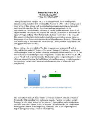
Introduction to pca v2
- 1. Introduction to PCA Christian Zuniga, PhD Friday, November 8, 2019 Principal component analysis (PCA) is an unsupervised, linear technique for dimensionality reduction first developed by Pearson in 19011,2,3. It is widely used in many areas of data mining such as visualization, image processing and anomaly detection. It is based on the fact that data may have redundancies in its representation. Data refers to a collection of similar objects and their features. An object could be a house and the features the location, the number of bedrooms, the square footage, and any other characteristic that can be recorded of the house. In PCA analysis, redundancy in the data refers to linear correlation among features. Knowledge of one feature reveals some knowledge of another feature. PCA may use this redundancy to form a smaller set of features, called principal components that can approximate well the data. Figure 1 shows the general idea. The data is represented as a matrix X with N objects (like houses) and F features (like square footage). PCA linearly transforms the features into a new set and retains the G most relevant features where G < F. The new features are called the principal components. The new data matrix Y is Y = PX, where P is a G by F projection matrix. The first principal component captures most of the variance of the data. Each additional principal component is made to capture the remaining variance and is uncorrelated or orthogonal to other principal components. Figure 1 PCA transforms a data matrix into a new one with fewer features. The cars dataset from UC Irvine will be used as an example4. This set contains 9 features for 392 cars of various makes and models. Figure 2 shows two sample features, ‘acceleration’ plotted vs. ‘horsepower’. Acceleration is given in the time taken for a car to accelerate from 0 to 60 mph. The figure shows the two features have opposite trends, or are negatively correlated. This is not surprising since higher horsepower should result in smaller times.
- 2. Figure 2 Two features of car data set shows the data is concentrated along a line P1. Figure 2 shows that most of the variation of the features is concentrated along a line labeled ‘P1’. The remainder of the variation is along a second line labeled ‘P2’. The lines can be characterized by unit vectors vj = [a1j, a2j] (j=1,2) that give the lines’ orientations. The lines’ displacements from the origin do not matter since the data will later be centered at zero. Each point represents a car and can also be represented by a vector xi = [horsepoweri, accelerationi], where the subscript corresponds to the ith car. Each point can be projected onto a line Pj by the inner product of vj and xi as shown in Figure 3. 𝑝!" = 𝑎!! 𝑎𝑐𝑐𝑒𝑙𝑒𝑟𝑎𝑡𝑖𝑜𝑛! + 𝑎!!ℎ𝑜𝑟𝑠𝑒𝑝𝑜𝑤𝑒𝑟! Figure 3 Projecting a point onto line P1. This new feature p1 is the first principal component and is a linear combination of the original two features, horsepower and acceleration. In general it will not have a more descriptive name but one could be given to clarify the concept. One option is to think of the combination of ‘horsepower’ and ‘acceleration’ as the ‘performance’ of the car.
- 3. The question is then how to find the coefficients a11, and a21 of vector v1, which gives the direction of the best-‐fit line P1. This line should be as close to all points as possible, minimizing the average distance J to all the points. 𝐽 = 1 𝑁 𝑑! ! ! !!! The solution lies in the covariance matrix of the features SX. Specifically; the eigenvectors of SX give the required vectors v1 and v2. To calculate the covariance matrix, the mean of each feature is subtracted from each row. To put the features on a similar scale, they should also be divided by their standard deviation. This is done to prevent the analysis from capturing uninteresting directions in the data. After this preprocessing of the data matrix X, the covariance matrix is and F by F matrix: 𝑺! = 1 𝑁 𝑿𝑿! The vector v1 corresponds to the eigenvector with largest eigenvalue λM. Vector v1 corresponds to the second smaller eigenvalue λm (λm < λM). 𝑺 𝑿 𝒗 𝟏 = 𝜆! 𝒗 𝟏 𝑺 𝑿 𝒗 𝟐 = 𝜆! 𝒗 𝟐 For the car data set, using only the features ‘acceleration’ and ‘horsepower’, the covariance matrix is. 𝑺 𝑿 = 1 −0.69 −0.69 1 The off-‐diagonal term -‐0.69 shows the cross-‐covariance between horsepower and acceleration, which is negative as implied by Figure 1. The diagonal terms show the auto-‐covariance of each feature and have value 1 because of the pre-‐scaling. Using any linear algebra solver readily gives the eigenvectors of the covariance matrix. The eigenvalues are (1.69, 0.31). Their sum is the total variance, which is 2. Vector v1 is [0.707, -‐0.707] and captures 84.5% of the total variance (1.69/2). Figure 4 shows the resulting directions of v1 and v2.
- 4. Figure 4 Rescaled data with the direction of the 2 principal components. The projection matrix P can be made with v1 and v2 as rows. If both vectors are kept, there is no loss in representation. The new representation would have a covariance matrix. 𝑺! = 1 𝑁 𝒀𝒀! 𝑺! = 1 𝑁 𝑷𝑿 𝑷𝑿 ! = 𝑷𝑺 𝑿 𝑷! = 𝚲 Since P has the eigenvectors of Sx as rows, the right hand side results in a diagonal matrix of the eigenvalues of Sx. 𝑆! = 1.69 0 0 0.31 For dimensionality reduction, only v1 would be used. The new representation, matrix Y, would have a single feature, the first principle component (Y = v1X). PCA can be applied to any number of features. The car data set has the additional features: ‘cylinders’, ‘displacement’, and ‘weight’ for a total of 5 features. Other features are categorical and one ‘mpg’ is usually the target variable of interest. The same process can be done to obtain the principal components. Each principal component is a linear combination of these 5 features. Standard scaling is applied on the features before making the covariance matrix Sx (now a 5 by 5 matrix). The eigenvalues and eigenvectors are found and the eigenvectors used to make the projection matrix P. Figure 5 shows the percentage of variance explained by each component. Again the first component captures over 80% of the total variance. Instead of 5 features, 1-‐2 principal components may be enough for various purposes.
- 5. Figure 5 Percentage of variance explained by each principal component. For example, Figure 6 shows a plot of principal component 2 vs. principal component 1. Together they capture about 96% of the total variance. The figure shows there may be 3 clusters, or groups of cars. These may correspond to different types of cars such as sports cars, sedans, and trucks. Confirming with the make of the car might clarify this. A clustering algorithm like k-‐means may be applied to quantify the clusters. This shows a common application of PCA in dimensionality reduction where fewer features help with many machine learning algorithms. Figure 6 Principal Component 2 vs. 1 indicates there may be around 3 clusters. To summarize, PCA is a linear, dimensionality reduction technique that forms new features using linear combinations of the original. These new features, the principal components, maximize the total variance capture and are uncorrelated with each other. The eigenvectors of the covariance matrix are used to transform the data matrix. In practice if there are many features, forming the covariance matrix may be computationally expensive and an SVD of the data matrix is used. [1] Gilbert Strang “Linear Algebra and Learning from Data” Wellesley Cambridge Press 2019
- 6. [2] Deisenroth, et. Al. “Mathematics for Machine Learning” to be published Cambridge University Press. https://mml-‐book.com [3] Shlens “A Tutorial on Principal Component Analysis” 2014 https://arxiv.org/abs/1404.1100 [4] https://archive.ics.uci.edu/ml/datasets/car+evaluation