This document summarizes the results of a helicopter electromagnetic survey conducted along a 130km pipeline corridor to map subsurface conductivity and aid in pipeline construction planning. The survey identified areas of shallow bedrock that would require blasting versus deeper overburden that could be trenched. Drill holes along the corridor were used to calibrate the electromagnetic conductivity measurements with actual subsurface conditions. A conductivity value of 6mS/m correlated well with a 2m overburden depth, the depth needed for pipeline trenching. The survey effectively mapped subsurface conditions and reduced costs associated with pipeline planning and construction.

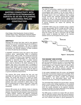
1. Greg Hodges, Chief Geophysicist, Geoterrex-Dighem
Jonathan Rudd, P.Eng., Geophysicist, Geoterrex-Dighem
Dominique Boitier, Compagnie General de Geophysique
ABSTRACT
Helicopter EM surveys have been used to map apparent
conductivity as an aid to characterizing ground conditions in
advance of pipeline construction. The cost of pipeline
construction is strongly dependent on the ground conditions
encountered, and accurate prediction of these conditions
can reduce the planning risk considerably.
A DIGHEM
V
conductivity survey was used to map ground
conditions along approximately 130km of prospective
pipeline corridor, 400m in width. The survey took about two
days to complete, providing a map of apparent conductivity
with a resolution of approximately 10m. The results are
interpreted to determine the extent of shallow bedrock
(which would require blasting) and deeper overburden
which could be trenched to the depth necessary for the
pipeline. Over much of the survey area it is possible to
define a single apparent conductivity value as the borderline
between soils, which could be trenched, and rock which
would have to be blasted. The survey maps the depth to
bedrock, and gives some indication of the soil types based
on ground conductivity measurements.
The airborne EM survey reduced the time and cost
associated with gaining land access and permission for
drilling. The survey also served as a check for buried,
unknown power lines and pipelines. Airborne EM surveys
have also been used to map ground conductivity after the
pipelines have been constructed to detect areas of high
ground conductivity due to clays or saline soils. These soils
can create conditions in which pipeline corrosion is
accelerated.
Airborne EM surveys are an effective means of reducing
cost and risk in the planning, construction and monitoring of
pipelines. Integrated with ground-based measurements and
a drilling program, airborne EM apparent conductivity
results can serve to gain a more complete understanding of
ground characteristics across the areas of interest.
INTRODUCTION
The costs of constructing a pipeline are highly dependant
on the relative occurrence of consolidated (rock) and
unconsolidated (soil) material in the top three metres of
ground. Where rock occurs in the upper 3 metres, it has to
be blasted which is far more expensive than trenching
through surficial soils. Helicopter electromagnetic (HEM)
surveys are used to map the electrical and magnetic
properties as an aid to characterizing ground conditions in
advance of pipeline construction. An accurate determination
of ground conditions can reduce the planning risk
considerably.
A DIGHEM
V
HEM survey was completed along a pipeline
corridor approximately 130 km in length and 400 m wide in
southern Quebec, Canada, as shown in Figure 1. The data
took four days to acquire. Drill results at several locations
along this corridor are used in conjunction with the HEM
survey results to delineate the depth of the interface
between soil and rock throughout the survey area.
Figure 1: Survey Area
THE DIGHEM
V
HEM SYSTEM
The Dighem
V
HEM system is a frequency domain system,
with five transmitter/receiver coil pairs in a bird slung below
the helicopter at a ground clearance of about 30m. The
standard system has a frequency range from about 380Hz
up to 56,000Hz, with coils oriented in both coplanar
configuration for high sensitivity resistivity mapping, and
vertical-coaxial coils for sensitivity to vertical conductors.
A new system developed since this survey, and designed
for this type of conductivity mapping work is available, which
employs 5 coplanar coil pairs with a frequency range up to
over 100,000Hz. This system provides more detailed
measurements in the near-surface layers, which will
improve the accuracy of this type of engineering survey.
The transmitted field energises the ground below, inducing
electric currents which change depending on the resistivity
of the ground. Variations in the soil and rock conductivity,
which are usually calculated as the apparent resistivity,
change the strength and phase relationship of the returned
secondary field measured with the receiver.
The HEM survey is carried out at about 30m per second,
with the HEM bird carried at about 30m ground clearance.
This survey speed provides for very rapid ground coverage,
and much reduced cost relative to ground geophysics on
MAPPING CONDUCTIVITY WITH
HELICOPTER ELECTROMAGNETIC
SURVEYS AS AN AID TO PLANNING
AND MONITORING PIPELINE
CONSTRUCTION

2. larger surveys. The entire 130km of pipeline corridor
surveyed for this project required only four days of data
acquisition. Increasing the width of the corridor surveyed
would only marginally increase the survey time, as it would
increase the size of each small block, improving the
efficiency of the survey process.
The system is positioned by real-time differential GPS, and
magnetic data and a video of the ground track are collected
with the EM. The magnetic data can help interpret the
changes in bedrock, as well as cultural interference. The
ground track video helps to verify position, and to identify
surficial features and culture. A 60Hz detector will identify
artificial power sources - power lines and buildings.
ELECTROMAGNETIC SURVEYS FOR
OVERBURDEN
The depth of exploration depends on several factors - the
frequency of the EM signal, the sensitivity of the receiver
and the conductivity of the ground. The penetration
increases as the EM frequency decreases. By employing
five different frequencies, the standard DIGHEM
V
system is
able to sample the ground at different depths, building a 3
dimensional picture of the distribution of resistivity in the
ground. For example, in ground of 100 mS/m conductivity,
the spread of frequencies will roughly sample between
surface and 60m deep. Sensitivity is controlled by the
quality of the electronics, and by the ability to see the weak
secondary field through the powerful primary field. The
DIGHEM systems accomplish this by moving the receivers
as far as practical from the transmitters, 8m. Decreasing
conductivity allows the EM fields to penetrate deeper into
the earth, increasing the depth of exploration (Fraser,
1978).
The strength of the anomaly depends on the conductivity
and thickness of the layers of overburden and geology. For
the purposes of this work, we are looking only at the near
surface, so we simplify the geology to overburden and
bedrock – two layers. Overburden is generally, although
not always, more conductive than the under-lying bedrock
(McNeill, 1980). This is due to the higher porosity and
hence higher water content of the overburden relative to the
bedrock, and to a generally higher content of electrically
conductive clay minerals in the soils. This is particularly true
of glacial tills, such as are common in the area of this
survey. Deeper overburden occupies a greater proportion of
the ground being sampled by the electromagnetic system,
and so creates a more conductive response than if the
system were sampling a higher percentage of bedrock.
In areas of relatively consistent overburden type, the
apparent conductivity measured can be correlated to the
overburden depth, and the shape of the conductivity
anomalies shows the distribution of the overburden.
The HEM system is complemented by a magnetic survey.
The magnetic data sets can be used in some cases to
discriminate conductive bedrock from conductive surficial
geology.
PROGRAM RESULTS
The results from two portions of the pipeline corridor are
discussed following. Block 22-26 represents approximately
8 percent of the surveyed corridor and block 12-13
represents approximately 4 percent. These areas were
chosen because they represent the areas for which drill
information was available.
Figure 2: Block 22-26
BLOCK 22-26
The first detail block covers a planned pipeline length of
approximately 11 km, surveyed as five linear segments. The
apparent conductivity from the 56,000 Hz coplanar EM data
set is presented over the topography in Figure 2. The
conductivity ranges from less than 1 to over 1000 mS/m.
Cultural features within planned pipeline corridors are
common since these routes are often planned along
existing infrastructure. The corridor which is presented here
runs through a relatively populated area and much of it
extends parallel with roads and transmission lines. The
56,000 Hz data set is relatively immune to these noise
sources and their effect is largely insignificant in the survey
results.

3. The general correlation of the conductive portions of the
surveyed area with low topographic relief supports the
interpretation that the variation in the conductivity is caused
primarily by conductive cover. A good example of this
correlation can be seen in the far north of the area, where a
stream with associated sediment causes a conductivity high
in the data set.
Conversely, topographic highs are generally seen to
correlate with conductivity lows. An interpreted bedrock
outcrop in the northern portion of the survey area and a
prominent topographic ridge in the south both produce
marked conductivity lows.
Exceptions to the general relationship of high conductivity
with thick soil cover are present in this area. A linear
conductivity high within the area indicated as a ridge, reflect
a conductive bedrock unit. The magnetic data sets can be
useful for the confirmation of bedrock sources, because the
magnetic data sets generally reflect bedrock sources only,
as surficial soils do not usually contain significant
concentrations of magnetic minerals.
Figure 3: Detail A
Drill hole information is available for two vicinities within this
block - within detail A and detail B. In detail A (see Figure
3), two drill holes have tested the boundary zone between
resistive bedrock to the west and conductive soils to the
east. The EM data sets indicate a conductivity of 5 to 6
mS/m for hole 57 and 4 to 5 mS/m for hole 52. These low
conductivities indicate a relatively thin layer of soil. Both drill
holes indicate a depth to bedrock of 1.5 m and depth to
water table of greater than 1.5m. At this shallow depth to
bedrock, the EM data sets are responding primarily to the
resistive bedrock beneath the soil. Toward the east, the soil
cover is interpreted to thicken significantly as indicated by
higher conductivities of 200 mS/m and more.
Two holes have been drilled in the detail area B (see Figure
4) where the topography slopes gradually toward the east
southeast. The two holes test an area where the EM data
sets indicate a moderately conductive response of between
5 and 15 mS/m. The first drill hole, 53, has an associated
conductivity of approximately 10 mS/m and has a depth to
bedrock of 3.35m. Hole 54 has an associated conductivity
of approximately 8 mS/m and a depth to bedrock of 1.75m.
Figure 4: Detail B
BLOCK 12-13
The second block covers a planned pipeline length of
approximately 5 km, surveyed as two linear segments. The
apparent conductivity from the 56,000 Hz coplanar EM data
set is presented over the topography in Figure 5. The
conductivity of this block is generally lower than Block A and
ranges from much less than 1 to approximately 100 mS/m.
Cultural features within this block occur in the central
portion through detail area C. A railway line, power
transmission line, and two roads extend from west to east
through this area. Again, the effect of these cultural features
is not significant in the 56,000 Hz data set and has little
bearing on the interpretation of the data set.
The topography in this block slopes gently downward from
the northern limit to the north-central portion of the area,
flattens to the middle of the area, and then slopes gently up
to the southern limit of the block. There is no general
correlation of the conductive portions of the surveyed area
with low topographic relief. Indeed, only three areas have
anomalously high conductivities indicative of significant
accumulations of soil. These three conductive areas are in
the extreme northeast of the area, across the central portion
of the area in detail A, and in the southern portion of the
area. The stream in the northern portion of the block does
have a correlating weak conductivity high, indicating some
accumulation of soils.

4. Figure 5: Block 12-13
The generally lower conductivity in this block suggests that
either the soils in this area are more sandy and therefore
less conductive, or that there is less soil cover.
Two holes have been drilled in the detail area A, where a
conductive feature in the EM data sets extends across the
Figure 6: Detail C
corridor. Hole 46 tests the centre of this conductive feature
where the apparent conductivity is 13 mS/m. The depth to
bedrock is quite deep at 8.35 m. Hole 45 tests the same
conductive feature, but on its southern flank. The apparent
conductivity at this location is 7 mS/m and the depth to
bedrock was found to be 4.95 m. The primary constituent of
the soil is till with near surface layers of silt, sand and
gravel. The water table is at surface.
As we expect, the decrease in conductivity (from 13 to 7
mS/m) correlates with a decrease in the thickness of the
surficial soils (from 8 to 5 m). This relationship will be
predictable where the conductivity of the surficial soils is
known to be relatively constant.
Figure 7: Conductivity vs. Soil Depth
CONDUCTIVITY TRENDS
The relationship between depth to bedrock and conductivity
is presented in graphical form in Figure 7. The general trend
in the data confirm that the conductivity increases with
increasing depth to bedrock. This trend is clear with 8 of the
10 drill holes. The remaining two holes, however, do not fit
this general trend.
Hole 29 has a low apparent conductivity of 7 mS/m and a
great depth to bedrock of over 20 m. This hole was drilled at
the edge of a large river bed where the major soil
constituent is sand. Very little clay is identified in the drill
logs. The absence of clay in the soil will serve to decrease
the overall conductivity and does, in fact, entirely account
for the low apparent conductivity in the EM response. In all
of the other drill holes, clay is a significant constituent of the
soil either as discrete layers or within till.
Hole 40 has a relatively low apparent conductivity of 10
mS/m and a depth to bedrock of 17 m. The hole was drilled
on the edge of a narrow, linear conductive feature which
reflects river sediments. The apparent conductivity is high
29
40
55
51
52
57
54
53
45
46
0
5
10
15
20
25
0
5
10
15
20
25
DEPTH TO BEDROCK
CONDUCTIVITY

5. because it is computed at the margin of the river bed and is
averaging the very low conductivity rock to the east with the
conductive soils in the river bed. The result of this averaging
is that the conductivity is understated.
We can look at these data in more detail by associating drill
holes which are in close proximity with each other, say
within a few hundred metres. In the figure, the data from drill
holes which are proximal to each other are joined by lines. It
is reasonable to expect that the closer the holes are to each
other, the less variation there will be in the composition of
the surficial soils. We would expect then, that for proximal
holes, the relationship between depth to bedrock and
conductivity would be better defined. This expectation is
confirmed in the three proximal hole pairs in Figure 7.
CREATING AN OVERBURDEN/BEDROCK
MAP
While the correlation between apparent resistivity and
overburden depth is affected by many more parameters
than just the depth of the overburden, in most cases the
overburden depth is the controlling factor on the apparent
resistivity of the near surface. The factors affecting the
direct relationship between overburden depth and apparent
resistivity are the type of overburden (which affects its
resistivity), the groundwater conditions and, to a lesser
degree, the bedrock type. Where these can be assumed to
be relatively constant, the overburden depth to conductivity
relationship will be predictable. This relationship can be
used to create a simple map distinguishing where the
overburden is deep enough for the pipeline trench to be
excavated by a backhoe, and where blasting will be
required. In the field, only a few drill holes along a very long
corridor for ground truth, or “calibration” of the results, can
allow a map to be created empirically, which can be used
for planning the pipeline route.
USING 2-LAYER INVERSION
In the case of this survey, it was found by comparison of
apparent conductivity to pre-existing drill holes that the
6mS/m (170 ohm-m) contour correlated quite well with a 2
metre depth of overburden, the depth of excavation needed
for the pipeline (Bouvier et al, 1999). This correlation was
established using only about a dozen drill holes, including
those previously described in this paper, over the 130km
length of the planned corridor. Any area with an apparent
resistivity of more than 170 ohm-m had insufficient
overburden to allow the pipeline to be placed without
blasting bedrock. If this correlation can be established
before the survey (from ground geophysics and test drilling,
for example), or in the field during the survey, it is possible
in the field to colour an apparent resistivity map to show two
basic colours, one for deep overburden and one for areas
which will require blasting.
In post-processing of the data, we use a multi-layer
inversion process to model the actual layer depth from the
highest frequency (Huang and Palacky, 1991). Such a map
is shown here in Figure 8. The map shows the depth to the
overburden in metres, derived by using a multi-layer
inversion of the 56,000 Hz data. The same features are
visible as were pointed out in the apparent resistivity map in
Figure 2, but now these features are measured in metres to
bedrock. The darkest black shows those areas for which
the interpreted depth to bedrock is less than the 2 metres
required for trenching with a backhoe. Also shown on the
depth map are the four drill holes on this segment of the
survey. The depths measured in the drill holes are within
0.5m of those measured from the HEM data inversion.
Figure 8: Depth to Bedrock
Because one frequency of the DIGHEM
V
system is highly
sensitive to this very shallow layer, the parameters inverted
must be limited, or the results will be unstable and the depth
section along the line will not be realistic. Where the soil
conductivity varies greatly over the area of the survey,
inversion parameters will have to be determined and
applied separately to different areas of the data. Any
additional information which can be used to define some
parameters of the inversion, such as overburden resistivities
measured with ground systems, can also be used to
improve the results. A DIGHEM
RES
resistivity system will
provide at least two frequencies sensitive to the near
surface, and an accurate inversion section can be
automatically calculated with corrections for variation in soil
conductivities.

6. Figure 9: Depth Section
It must be recognized that these results are derived from a
system 30m in the air, moving at 30m/s. At that altitude, the
system has a footprint of about 50 to 100 metres, so there is
a certain amount of averaging of the actual depth, and limit
to the resolution (Kovacs et al, 1995). A single drill hole may
not match the measured value from the HEM because of
the difference in sample size. This was demonstrated earlier
in the description of hole 40, Figure 7, where the hole was
on the edge of a bedrock ridge. If the HEM were matched to
a statistical average of many holes spaced only a few
metres apart, the match may be much more meaningful.
The accuracy of the results is also dependent on the
consistency of the match between the model(s) used in the
inversion and the ground conditions. While enough follow-
up information was not available to the authors to create a
statistically meaningful comparison of the predicted depths
and the final overburden depths measured during
construction, the results appear to have been accurate to
approximately 0.5m in the upper 3m. While this may not be
accurate enough to exactly define locations and depths at
which blasting must be used, it is sufficient to define the
total amount of blasting necessary, the locations at which it
clearly will or will not be needed, and preferable routes to
avoid bedrock. In areas where the indicated depth of
overburden is clearly much greater, or much less than the
planned depth only a few confirmatory drill holes will be
needed, to establish the margin of error. In transitional
zones between deep and shallow overburden closely
detailed drilling will be necessary to identify exact zones
through which trenching will suffice.
If we can create a depth to bedrock map like Figure 8, then
we can also create a depth section. Figure 9 shows a depth
section, demarcating bedrock from overburden, for the
central survey line through block 22-26 shown in the depth
map. Note that there is considerable vertical exaggeration
necessary to show the bedrock depths. We have also
indicated on the section the planned depth of the pipeline,
so the presentation makes it relatively easy to see where
the bedrock depths are marginal, or definitely too shallow
for backhoe trenching.
When actually planning the pipeline corridor, an airborne
resistivity / overburden depth survey is the fastest method of
mapping the overburden conditions over a wide corridor. A
broad area of prospective ground can quickly be mapped to
identify the ideal pipeline route to minimize cost and
environmental disruption.
POST-CONSTRUCTION SURVEY
The survey we have shown was conducted in advance of
any construction. However, the existence of a pipeline does
not prevent a survey from being conducted to map the soil
resistivity or depth. The example in Figure 10 shows a
survey conducted along a 25km section of the Trans
Canada Pipeline in central Canada, to map soil salinity.
The purpose of the survey was to identify highly conductive
soils close to the pipeline, as they increase the risk of
corrosion of the pipeline. The depth of overburden was
great enough that depth was not a factor affecting the
measured apparent resistivity. In this survey two main
Figure 10: Post-Construction Surveys

7. zones of higher conductivity are apparent, marked at A and
B. Zone A correlates to an area where increased soil
salinity is known. (TCPL, Pers comm, 1997) The source of
the increased conductivity at B is not known.
ACKNOWLEDGEMENTS
The authors gratefully acknowledge Entrepose Ltd. for
permission to show the data from this survey, and for the
drill information presented here. We also thank Trans
Canada Pipelines Ltd. for permission to show their data.
The variations in apparent resistivity show that the this can
be measured close to existing pipelines, in this case a
corridor containing several 30” to 40” pipelines several
metres apart. The pipelines do affect the data on flight lines
within about 50m, but outside that corridor the soil resistivity
is accurately mapped.
REFERENCES
Bouvier, A, Elkaim, P., Hodges, G., 1999, Heliborne
Electromagnetic & Magnetic Surveying Applied to a Pipeline
Construction Project in Canada. Presented at EEGS
Annual Meeting, Budapest.
Fraser, D.C., 1978a, Resistivity mapping with an airborne
multicoil electromagnetic system: Geophysics, v. 43, p. 144-
172.
Huang, H, and Palacky, G.J., 1991; Damped Least-Squares
Inversion of Time-Domain Airborne EM Data Based on
Singular Value Decomposition Decomposition. In
Geophysical Prospecting, Vol 39, pp 827-844, 1991
Kovacs, A., Holladay, J.S., Bergeron, C.J, 1995, The
footprint/altitude ratio for helicopter electromagnetic
sounding of sea-ice thickness: Comparison of theoretical
and field estimates. Geophysics, Vol 60, No. 2, March-April
1995
McNeill, J.D. 1980, Electrical Conductivity of Soil and
Rocks. Geonics Technical Note TN-5. Geonics Ltd,
Mississauga, Ontario, Canada