2. (a) (b)
(c)
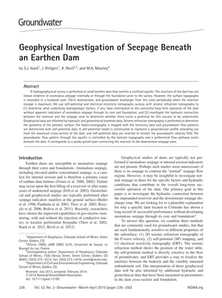
Figure 1. Description of the field site. (a) 1:24,000 topographic map of field site showing survey area, seepage location and
position of site photos relative to the dam crest and reservoir (map published by USGS, 1965 and inspected/revised 1994,
reference code 39105-G2-TF-024). (b) Photo taken on the dam crest at the south abutment facing northeast towards location.
(c) Photo taken on profile P7 facing west toward the toe access road and the dam crest.
Description of the Test Site
Localization and Geometry
The field site is a homogeneous earth-fill dam located
at the base of the Rocky Mountain foothills in Jefferson
County, Colorado. The topography is shown in Figure 1a
and photos of the dam crest from the right (south)
abutment and the maximum cross-section of the dam are
shown in Figure 1b and 1c. The topographic gradient
within the survey area is mild and points towards the east
at the center of the dam crest. The topographic variability
in a N-S direction along the strike of survey profiles P1-P6
is minor. A 1:3,600 aerial photograph of the survey grid
and the reservoir geometry is given in Figure 2. The dam
is 3.7 m wide at the crest and 427 m long, and is composed
of homogenous earth fills directly borrowed from onsite
materials excavated from the reservoir basin (Denver
Water 1988). It is 4 m tall at the maximum cross-section
and the hydraulic height is 3.7 m. The upstream and
downstream slopes have a 2.5:1 grade. The impounded
reservoir (Figure 2) stores a maximum of 3.60 × 10⁵ m3
of water at the high maximum pool elevation of 1800.4 m.
The normal storage elevation of the reservoir is 1800.1 m.
At this elevation the reservoir surface area is 1.1 × 10⁵
m2
and the storage capacity is 2.5 × 10⁵ m3.
Geology and Geotechnical Properties
The reservoir lies entirely within the upper portion of
the Laramie formation, although the west and southwest
reservoir rims are faulted against the impermeable Pierre
shale formation (Denver Water 1988). The engineering
Figure 2. Aerial photo of the survey area showing the
location of access roads and the downstream seepage zone.
The dam is 3.4-m high and positioned between the toe access
road and the crest access road at the cross-section of profile
P7. Station markers represent the position of the electrodes
for the electrical resistivity tomography and the self-potential
(white filled circles) and the two seismic tomography field
stations (red lines). Profile P2, positioned at the toe between
profiles P1 and P3, has been omitted for clarity.
design records for the dam describe the site as a four layer
system composed from top to bottom of (1) a maximum
of 4 m of embankment fill compacted to 94% of the
standard Proctor maximum dry density, (2) a layer of
sandy to very sandy “natural” unconsolidated clay that
NGWA.org S.J. Ikard et al Groundwater 53, no. 2: 238–250 239
3. Table 1
Model Parameter Summary for Modeled Soil
Textures
Property
Natural
Clay Aquifer Bedrock
Percent gravel1 (% wt.) 0.00 50.0 0.00
Percent sand1
(% wt.) 32.0 18.0 32.0
Percent silt1 (% wt.) 24.0 0.00 24.0
Percent clay1
(% wt.) 44.0 32.0 44.0
Compaction1 0.94 0.94 1.18
Residual water content2
(% vol), θr
26.2 11.1 26.2
Porosity2
(−), φ = θs 0.49 0.43 0.36
Hydraulic conductivity2,3
(mm/hr), Ks
2.0 5.0 0.04
Bulk density2
(kg/m3
), ρ 1,360 1,510 1,690
van Genuchten parameter2
α (m–1
)
0.36 5.7 × 10⁻³ 3.0 × 10⁻³
van Genuchten parameter2
n (−)
1.4 0.73 0.93
Formation factor4
(−), F 6.0 8.3 12.9
Excess charge density5
(C/m3
), QV
9.89 2.91 1864
Bulk conductivity6
(mS/m), σ
8.2 5.9 3.8
ηf denotes the dynamic viscosity of the pore water (10–3 Pa s at 25◦
C).
1From borehole grain size distribution data supplied by the dam owner.
2From SPAW soils database of Saxton and Rawls (2006).
3Based on prior geotechnical tests.
4Using F = φ–m with m = 2.5 for clayey sediment (Revil et al. 2012).
5Using C = −QV kρf g/ σηf , where σ = σf /F with σf = (4.9 ± 0.2)
× 10–2 S/m (pore water conductivity).
6Using for the bulk conductivity σ = σf /F with σf = (4.9 ± 0.2) × 10–2 S/m
at 20◦
C.
is 0.6 to 2.3 m thick, (3) a layer of silty/clayey sandy-
gravel that is 1.4 to 2.7 m thick, and (4) the impermeable
claystone bedrock of the Laramie formation (bedrock)
(Denver Water 1988). Bedrock was encountered beneath
the dam crest in exploratory holes at shallow depths (4.0
and 6.9 m). The permeability of the silty/clayey sandy-
gravel layer above the bedrock is reported to be two orders
of magnitude greater than that for the bedrock, and one
order of magnitude greater than the permeability of the
overlying unconsolidated clay sediments (Table 1). The
clayey sandy-gravel layer appears therefore as an aquifer
confined by the overlying and underlying impermeable
horizons. This aquifer has been partially to completely
exposed in the reservoir basin during construction of the
reservoir and dam.
Grain size distributions from samples collected in
three exploratory boreholes (see position in Figure 2) will
be used later to parameterize the flow equation during
forward and inverse modeling. The boreholes were com-
pleted at the north abutment, the center of the dam crest,
and at the south abutment. Samples were available from
depths between 0.6 and 5.5 m, and represent all of the
layer horizons above the impermeable bedrock. The mass
percentages of the coarse and fine fractions are shown in
Figure 3 and confirm the hydrostratigraphic units existing
above the bedrock. We assume that the embankment and
natural clay horizons have similar grain size distributions
because the embankment was constructed from the
natural clay materials that were excavated from the
reservoir basin. Thus, the unconsolidated natural clay
horizon is represented by the grain size distributions that
correspond to depths less than 3.0 m that have a much
greater fines fraction than samples from greater depths.
The mean coarse fraction (sand plus gravel) of these
samples is 32 ± 10%, and the mean fines fraction (clay
plus silt) is 68 ± 10%. The samples collected at depths
greater than 3.0 m represent the sandy-gravel aquifer and
have significantly increased coarse fraction. The mean
coarse fraction of these samples is 82 ± 10% by mass.
We used hydrometer analyses of samples collected
between 1.8 and 3.0 m to determine the percentage of
silt and clay present in the fines fractions shown in
Figure 3. The resulting mass fraction gradation of the
embankment and natural clay horizons consisted of 0%
gravel and organic matter, ∼32% sand, ∼24% silt, and
∼44% clay. The mass fraction gradation determined for
the sandy gravel layer underlying the embankment and
natural clay horizons is ∼50% gravel, ∼32% sand, and
∼18% clay. Soil-water retention parameters for a two
parameter van Genuchten-Mualem model (van Genuchten
1980) were estimated from these data by entering the
mass fraction distributions of each horizon into the Soil
Plant Air Water (SPAW) database described by Saxton
and Rawls (2006). The resulting soil-water retention
curves were then fitted by iteratively adjusting the model
parameters. The Saxton and Rawls (2006) database also
provided statistical estimates of bulk density and saturated
hydraulic conductivity which were used to compute the
porosity and intrinsic permeability for each horizon above
the impermeable bedrock. The bulk densities compare
well with the 94% of maximum dry density estimated
Figure 3. Mass fraction constituents of samples collected
in boreholes determined from grain size distributions. The
layer below 3.0 m corresponds to the confined aquifer. The
permeability of the aquifer is one order of magnitude
greater than the overlying natural clay and three orders of
magnitude greater than the underlying bedrock aquitard.
240 S.J. Ikard et al Groundwater 53, no. 2: 238–250 NGWA.org
4. earlier. The parameters of the bedrock (rich in smectite)
were estimated by assuming a permeability that was
three orders of magnitude less than the clayey sandy-
gravel aquifer. All of the geotechnical values described
previously are summarized in Table 1.
Anomalous Seepage
Anomalous seepage was not observed or detected
through the cross-section or foundation of the dam prior
to the survey. However, a localized zone of surface soil
mounding is present between 150 and 180 m downstream
of the dam, with significantly greater soil moisture
content than surrounding topography (see localization
in Figure 2). Furthermore, groundwater discharge has
been observed in this zone and correlated with the peak
reservoir levels.
Hydrogeophysical Investigations
The primary goal of our study was to investigate the
hydraulic connection between the impounded reservoir
and the downstream seepage discharge zone, and to pro-
vide a plausible explanation for why the dam has shown
a long record of successful performance without develop-
ing anomalous seepage through its core and foundation.
The P-wave velocities and electric conductivities increase
in each successive layer at depth, and the self-potential
is directly sensitive to groundwater flow, therefore these
methods are ideal for such an investigation. The sur-
vey layout for seismic, self-potential, and ERT profiles
is shown in Figure 2.
Seismic P-Wave Tomography
Two 2D seismic profiles, S1 and S2, were collected
with a 24 channel SeimicSource DAQ Link III using
a 0.25 ms sample interval and twenty four vertical axis
4.5 Hz center-frequency geophones. Seismic profile S1
was established along the dam center line perpendicular
to the crest inline with ERT profile P7 (Figure 2), and
seismic profile S2 was established at the toe parallel to the
crest between ERT profiles P2 and P3. Geophones were
spaced 2 m along these profiles, and a seismic source was
traversed every 4 m along the profiles and provided by
dropping a 5.4 kg (12 lb) sledgehammer onto an aluminum
plate from an elevation 1.5 m above the surface. Seismic
sources were positioned with zero-offset from a given
receiver location for each shot. Travel times of head waves
refracted from the phreatic surface were observed at each
station and inverted to recover the 2D distribution of
P-wave velocity in the subsurface beneath each of the
profiles.
Example raw seismic shot gathers are shown in
Figure 4a and 4c with the interpreted first arrivals
indicated on these figures as red lines. An interpretation
of observed shot gathers for profile S2 is also included in
Figure 4b. The travel-time data were preprocessed prior
to performing the inversion, as described below. First
arrival times of the P-wave wave energy in each shot
gather were selected using the built-in module in the
Vscope data acquisition software that was used during
the acquisition. A floating pretrigger delay was used
during data acquisition, and the relative “time-zero” for
each shot gather was determined by the onset of seismic
energy at the zero-offset receiver for each shot. This
arrival time was then subtracted from each pick for a
given shot gather to obtain relative arrival times for use
in tomographic modeling. 2D travel-time tomography of
the P-wave velocity distribution was performed with the
SeisOPT2D software which employs a synthetic annealing
algorithm in conjunction with a stochastic Monte-Carlo
procedure to find a velocity model that yields a global
minimum value of the root-mean-square error between
the observed travel-time data and forward calculated data.
Velocity constraints were not applied to the model during
the inversion procedure, however, the resultant modeled
velocities are well within reasonable values for the present
hydrogeological setting, offering validity significant to the
final obtained velocity model. The inversion results of the
two profiles S1 and S2 are shown in Figures 5 and 6.
Self-Potential Data
A larger survey consisting of 2D ERT and self-
potential profiles was completed at the field site between
March and June 2011, the same time period when seismic
refraction data was collected. The survey consisted of
seven 2D profiles collected on the dam crest, downstream
slope, and the downstream topography. Crest-parallel
profiles P1-P6 began south of the dam centerline and were
terminated adjacent to the left (north) abutment. Data were
collected along profile P5 at two different times during
the survey period and were offset by one 16 takeout cable
reel between each survey. Crest-perpendicular profile P7
began at the reservoir surface contact on the upstream
slope at the dam centerline, and extended 280 m out
into the downstream topography. The electrode spacing
along all profiles was 5 m. Profiles P1-P3 were offset
horizontally in a downstream direction by 10 m, and
profiles P4-P6 east of the access road were offset by 30 m.
A total of 778 self-potential stations were measured at
the field site using two nonpolarizing Pb-PbCl2 electrodes
and a handheld Fluke 289 true RMS digital multimeter.
A reference electrode was buried in an excavated pit near
the right abutment of the dam (Figure 2) and assigned
a potential of 0 V. All measured self-potential data were
adjusted to be relative to this reference electrode. At
each station, a shallow hole was excavated to expose soil
moisture and reduce the contact resistance between the
electrode and the ground. The minimum and maximum
resistances for the survey were 1 and 130 k (measured
with the voltmeter), respectively, and the mean resistance
for all stations was 20 k , well below the internal
impedance of the voltmeter (100 M ). The potential dif-
ference between the reference and roving electrodes was
measured before and after acquiring data along each 2D
profile, and the electrode drift was computed and removed
from each profile during processing. The electrical con-
ductivity of the reservoir water was measured during the
survey and was σf = 457 μS/cm–1
(0.046 S/m) at 25◦
C.
NGWA.org S.J. Ikard et al Groundwater 53, no. 2: 238–250 241
5. (a)
(b)
(c)
Figure 4. Seismic shot gathers. (a) Raw shot gather for seismic profile 1 collected along the dam crest with P-wave arrival
time picks plotted as red lines. First arrival picks were used for the inverse tomographic modeling. (b) Graphic interpretation
of a shot gathered from profile S2. (c) Shot gather for seismic profile S1.
DC Resistivity Data
Resistivity data were collected using an ABEM Ter-
rameter 4000 LUND imaging system with a Wenner-64
array protocol. The measured resistances along each
profile were used to produce 2D pseudo-sections of the
apparent resistivity distribution beneath each profile.
Pseudo-sections were inverted in 2D with RES2DINV
using a finite-element approach (Loke and Barker 1996).
The topography has been taken into account in the
inversion but is negligible in the parallel profiles. The
topography is accounted for in the inversion of the per-
pendicular profile and is included in the inverted results.
Interpretation of the Geophysical Data
Seismic P-Wave Tomography
The inverted P-wave velocity models and the corre-
sponding ray-path coverage are shown in Figures 5 and
6. Warm colors (yellows and reds) indicate high veloc-
ity zones and dense ray-path coverage, while cool col-
ors (greens and blues) represent low velocity zones and
reduced ray-path coverage. Because of dense source loca-
tions along each line, the ray-path coverage is relatively
dense, and the inverted velocities are relatively well con-
strained within the model space. Piezometer locations and
242 S.J. Ikard et al Groundwater 53, no. 2: 238–250 NGWA.org
6. (a)
(b)
Figure 5. P-wave velocity inversion results for seismic profile 1 (S1) collected parallel to the crest along the downstream toe
of the dam. (a) P-wave velocity distribution. Color scale indicates seismic velocity. (b) Ray-path coverage density plot showing
a relative sensitivity distribution. Color scale represents the number of rays that intersect a given model element or pixel.
The intersections with ERT profile P7 and seismic profile S2 are indicated at the top of the tomogram.
the interpreted depths to the water table are shown on
the figures as well. The interpreted position of approx-
imately 95 to 98% water saturation within the capillary
fringe (black-dotted line) has been interpolated between
the piezometers and within the dam based on the measured
water table depths and the inverted velocity distributions.
It is worth noting that the seismic refraction method is
sensitive to the level of water saturation, and can there-
fore be used to image the capillary fringe (Bardet and
Sayed 1993). P-wave velocities become sensitive to sat-
uration levels above approximately 95%, and this can be
seen in the tomograms as a sudden increase in veloc-
ity within the immediate vicinity of the water table as
measured in piezometers along the seismic profiles. The
interpreted depth to greater than 95% saturation increases
sharply in the downstream half of the dam, correspond-
ing to flow conditions in good agreement with the strong
negative self-potential anomaly observed beneath the crest
on profile P7 (Figures 7 and 8) (see Titov et al. 2005, for
a modeling of this effect). The velocity of the saturated
clayey sandy-gravel aquifer (indicated by the solid-black
lines in Figures 5 and 6) is much higher than that of the
overlying unconsolidated natural clay sediments, and is
in good agreement with typically assumed P-wave veloc-
ity ranges for saturated shales and clay sediments (1100
to 2500 m/s). The capillary fringe is resolved above the
phreatic surface in the velocity range 600 to 1100 m/s. The
velocity distribution beneath the dam crest seems homo-
geneous in the embankment above the phreatic surface,
and shows little to no lateral variations in the natural clay
sediments below the water table. The observed increase in
P-wave velocity with depth is the result of increased satu-
ration and decrease in porosity, from unconsolidated clays
to more compact aquifer sediments into the compacted
bedrock, and the depths of the sharp velocity interfaces
observed in the tomograms are in good agreement with
the depths of these layers interpreted from the grain size
distributions and ERT (Figures 7 and 8).
Resistivity and Self-Potential Data
Figures 7 and 8 show 2D electrical resistivity
tomograms collected across the crest and perpendicular
to the crest at the dam centerline, and the corresponding
self-potential data along each profile. The resistivity
tomograms show each of the layers observed in the
geotechnical boreholes and P-wave velocity distributions
at depth, and show an increased thickness of the upper
natural clay layer due to the presence of the embankment
materials, which are assumed to be a slightly disturbed
version of the natural clay horizon as explained above.
The subsurface electric conductivity increases with depth.
The embankment dam and unconsolidated natural clay
layers have resistivities greater than 50 m. The highly
conductive, impermeable, claystone bedrock aquitard is
NGWA.org S.J. Ikard et al Groundwater 53, no. 2: 238–250 243
7. (a)
(b)
Figure 6. P-wave velocity inversion results for seismic profile S2 normal to the dam crest. (a) P-wave velocity distribution.
(b) Ray-path coverage density plot, showing a relative sensitivity distribution. The color scale of the ray-path coverage plot
represents the number of rays that intersect a given model element or pixel. Here, the approximate embankment/foundation
contact is plotted as a black-dashed line, and the intersections with ERT profiles P1, P2, and P3, and seismic profile S1
are indicated at the top of the tomogram. Along both profiles S1 and S2, the black-dotted line indicates the depth at which
the saturation levels within the capillary fringe begin to affect the P-wave velocity (saturation ∼95%). The solid-black line
indicates the interpreted phreatic surface. The average 2011 water table elevations from piezometer data are plotted as white
triangles/lines. The maximum and minimum water elevations recorded during 2011 are plotted as black triangles.
characterized by low resistivities (less than 10 m). The
ERT data suggest that the aquitard surface is undulatory
beneath the dam crest (see Figure 7) in a crest-parallel
direction and approaches the surface downstream of
the dam centerline along profile P7 (see Figure 8)
perpendicular to the crest.
A general methodology to interpret self-potential
signals can be found in Jardani et al. (2007) and the
reader would find details regarding the underlying
physics in Titov et al. (2002) and Revil et al. (2012). The
self-potential data are sensitive to groundwater flow in the
subsurface, and the self-potential anomalies are therefore
significantly spatially correlated with the bedrock surface
topography that is observed in the 2D ERT profiles.
Self-potential data observed along the dam crest are pre-
dominantly negative with respect to the reference station
and indicate a relatively strong component of ground-
water seepage oriented vertically downward beneath and
through the dam cross-section (see Figures 7 and 9).
About 93% of the 315 self-potential stations measured
along the dam crest showed self-potential readings less
than 0 mV relative to the reference electrode. In contrast,
the self-potentials observed downstream of the dam along
profile P7 are primarily positive relative to the reference
electrode, indicating that groundwater flow is directed
predominantly upward towards the surface. About 97% of
self-potential measurements along profile P7 are greater
than 0 mV relative to the reference electrode, and the
only negative self-potential anomaly observed along this
profile corresponds to stations measured on the dam crest
and downstream slope. The increasing and decreasing
trends in the self-potential data corresponding to profile
244 S.J. Ikard et al Groundwater 53, no. 2: 238–250 NGWA.org
8. Iteration 5, RME error 6.0%
Elecrical resistivity (Ohm m)
1810
1800
1790
1780
1770
1760
1750
Electrical resistivity tomogram
Self-potential profile P1
Dam and natural clay material - Aquifer
Claystone bedrock - aquitard
20
15
10
5
0
-20
-15
-10
-5Elevation(m)Self-potentialsignals(mV)
Distance along the profile (m)
SOUTH NORTH
Reference potential
P7
(b)
(a)
0.0 50
5.0 10 20 50 100
100 150 200 250 300
Figure 7. Electrical resistivity tomography and self-potential measured on the crest (profile P1, taken at the crest of the dam).
(a) Self-potential data on the crest were predominantly negative with respect to the reference electrode and were showing
very small spatial fluctuations with respect to those shown in Figure 8. (b) Electrical resistivity tomogram across the crest.
The aquifer-aquitard boundary corresponds to the dash line.
P7 are spatially correlated with the bedrock peaks
and troughs observed in the corresponding ERT data,
respectively, and, excluding the first station (measured in
the reservoir water) and the positive anomaly observed in
the three stations at the eastern-most end of the profile,
the largest positive self-potential anomalies are positioned
over the two bedrock peaks in the observed seepage zone
150 to 180 m downstream of the dam. For each bedrock
peak observed in this zone, the self-potential signal
becomes more positive (in a downstream direction) on
the upstream side indicating groundwater is being chan-
neled towards the surface on the upstream slope of the
seepage zone, and then decreases (also in a downstream
direction) on the downstream slope as the groundwater is
being channeled vertically downward to greater depths.
Some of the groundwater in this vicinity intersects the
surface and results in the observed seepage at the ground
surface, and a significant volume of the groundwater in
this zone is also bifurcated around these bedrock peaks,
as indicated by the strong negative self-potential anomaly
A8 (see Figure 9a).
The self-potential data are shown in relation to
the surface and bedrock topography in Figure 9 and
illustrate the high degree of correlation of positive
and negative anomalies with peaks and troughs of the
bedrock surface. Negative anomalies are shown in shades
of green and blue and are representative of flow zones,
but do not necessarily reflect vertical flow. The negative
anomalies tend to be positioned over bedrock troughs that
create continuous preferential flow channels through the
subsurface. The most negative self-potential anomalies
are shown along the dam crest (anomaly A1), and at the
south end of profile five (anomaly A8). These negative
anomalies are associated with flow through the bedrock
trough beneath and parallel to the dam crest (anomaly
A1), and the zone of groundwater bifurcation around the
bedrock mounds observed in profile P7 (anomaly A8).
Additional negative, albeit lesser amplitude, anomalies
are also observed downstream of the dam and provide
an indication of preferential groundwater flow channels
through the aquifer that are formed by the bedrock
troughs. Anomaly A2 at the north abutment is a reflection
of flow that is being channeled through a bedrock trough.
Anomalies A4, A5, and A6 reflect the same, and are
interpreted to result from groundwater flow through a
continuous path that is formed by a bedrock trough and
intersects the bedrock slope at the southern-most end of
profile P5 that produces anomaly A8.
The self-potential anomalies are predominantly pos-
itive downstream of the dam, and in contrast to the
negative anomalies, the positive anomalies indicate that
much of the groundwater flow beneath the dam is being
NGWA.org S.J. Ikard et al Groundwater 53, no. 2: 238–250 245
9. Iteration 5, RME error 5.1%
Elecrical resistivity (Ohm m)
Electrical resistivity tomogram
Aquifer
Claystone bedrock - aquitard
Elevation(m)
Distance along the profile (m)
1800
1790
1780
1770
1760
1750
Seepage and surface mounding
Dam
crest
Self-potential profile P7
Self-potentialsignals(mV)
Positive anomaly
Dam toe
Infrastructure
30
20
10
0
0.0
5.0 10 20 50 100
40 80 120 160 200 240
-10
-20
Outlier
WEST EAST
Reference potential
P1
(a)
(b)
Figure 8. Profile P7 normal to the dam crest and intersecting the seepage zone 150 m downstream of the dam. (a) Self-potential
profile. The positive anomaly at the west end of the profile was measured at the contact between the upstream dam slope and
the reservoir. A negative self-potential anomaly is present beneath the dam crest as reservoir water is channeled through the
clayey-gravel aquitard below, and increases at the dam toe as seepage is channeled upward to a local bedrock plateau created
when the reservoir basin was constructed. (b) Resistivity tomogram of Profile 7. The aquifer-aquitard boundary corresponds
to the dash line.
channeled vertically in a direction towards the surface.
The trend of negative self-potential beneath the dam to
predominantly positive self-potential downstream of the
dam is consistent with the shallowing bedrock surface
geometry shown in 2D ERT profiles (not shown here).
The large positive anomaly A3 occurs in a zone where the
bedrock is a shallow plateau that is relatively planar and
free of undulation and troughs. Anomaly A7 is positioned
over the downstream discharge zone associated with the
bedrock mounds shown in 2D ERT profile P7, and con-
sists of two spatially localized, strong positive anomalies.
Each individual anomaly is correlated with the one of the
bedrock mounds, and both show a reduction in amplitude
immediately downstream of the associated mound. The
source of anomaly A9 is currently unknown. This anomaly
is in the vicinity of drainage infrastructure at the southeast
boundary of the survey area (see Figures 1 and 2), or may
also result due to bedrock outcropping in the vicinity.
A 3D representation of the bedrock surface in the
survey area was constructed by kriging the (x, y, z)
coordinates that were hand-picked from the bedrock
surfaces shown in the 2D ERT profiles. The self-
potential data is displayed over the bedrock surface
topography Figure 9b to emphasize the anomalies that
are spatially correlated with the greater bedrockpeaks
and troughs. Self-potential anomalies are shown to be
highly correlated with the bedrock topography. Negative
self-potential anomalies are correlated with the greatest
bedrock surface depths, as well as on the downstream
slopes of bedrock peaks and plateaus, and the positive
self-potential anomalies are generally associated with the
upstream slopes of bedrock peaks and on plateaus, where
groundwater is flowing vertically upwards.
Laboratory Investigation
A sample of sediment was collected from the
reservoir bed at the south abutment during a low pool
condition, shortly after the survey was completed. A
sample of reservoir water was also collected to use
with the sediment in quantifying the streaming potential
coupling coefficient connected the electrical potential to
the hydraulic heads. Data were obtained by installing
the material at the base of water column, and filling the
column with the sample of reservoir water. The water
column containing the sample was then positioned in
another reservoir containing the water collected from the
dam, to establish a hydraulic gradient across the sample.
The sediment sample was allowed to achieve equilibrium
with the water in the column and the reservoir for 48 hrs
prior to performing the experiment. The hydraulic gradient
246 S.J. Ikard et al Groundwater 53, no. 2: 238–250 NGWA.org
10. (a)
(b)
Figure 9. Self-potential data (in mV) at the field site. (a)
Self-potential data with topography showing the downstream
slope of the dam and downstream topography. A1 to A9
represent characteristic anomalies that are discussed in the
main text. (b) Self-potential data with bedrock topography
determined from electrical resistivity tomography.
in the experimental apparatus was varied in time and the
potential difference across the sample was measured as a
function of the hydraulic gradient with two nonpolarizing
Ag-AgCl electrodes and a Fluke 289 digital multimeter.
The streaming potential coupling coefficient C is the
key parameter controlling the amplitude of the self-
potential signals for a given head gradient. We found
C=−0.7 ± 0.2 mV/m, a value consistent with the trend
between C and the pore water conductivity shown by
Revil et al. (2003, their Figure 3).
Forward and Inverse Modeling of the
Self-Potential Field
A 2D steady-state numerical model of coupled elec-
tric and groundwater flow was constructed in COMSOL
Multiphysics 4.3a to model the self-potential data and
their relation to seepage along profile P7 perpendicular to
the crest at the dam centerline. The geometry and depths
of the bedrock and aquifer layers of the model space were
obtained from ERT data acquired along profile P7. The
self-potential signals that were recorded in the field were
modeled and inverted to recover the 2D distribution of the
causative electrical current sources within the dam and
subsurface. The inverted electrical current sources were
used to quantify the Darcy velocity, as described below
(see Soueid Ahmed et al. 2013, for additional tests of this
methodology).
Computation of the Prior Groundwater Flow Model
For the hydraulic problem we solve the governing
Richards equation (Richards 1931),
[Ce + SeS]
∂H
∂t
+ ∇· [−K∇ (H + z)] = 0, (1)
where z is the elevation head (m), H is the total
hydraulic head (m), Ce denotes the specific moisture
capacity (in m–1
) defined by Ce = ∂θ/∂H where θ
is the volumetric water content (dimensionless), Se is
the effective saturation of the medium (dimensionless),
related to the relative saturation of the water phase by
Se = Sw − Sr
w / 1 − Sr
w (θ = Swφ where φ represents
the connected porosity of the soil material), S is the
storage coefficient (m–1
), and t is time. The hydraulic
conductivity K is related to the relative permeability
kr and the hydraulic conductivity at saturation, Ks,
by K = krKs. The effective saturation, specific moisture
capacity, relative permeability, and the volumetric water
content are defined by (van Genuchten 1980),
Se =
1/ 1 + |αH |n m
, H < 0
1, H ≥ 0
, (2)
Ce =
⎧
⎨
⎩
αm
1−m (φ − θr) S
1
m
e 1 − S
1
m
e
m
, H < 0
0, H ≥ 0
(3)
kr =
⎧
⎪⎨
⎪⎩
Sl
e 1 − 1 − S
1
m
e
m 2
, H < 0
1, H ≥ 0
(4)
θ =
θr + Se (φ − θr) , H < 0
φ, H ≥ 0
(5)
where θr denotes the residual volumetric water content
and α, n, m, and l (m = 1 – 1/ n) are material proper-
ties. Equation 1 was parameterized with statistically based
estimates of saturated hydraulic conductivity, bulk den-
sity, residual and saturated moisture contents, and soil-
water retention curves corresponding to a clay textured
soil. These estimates were obtained by fitting soil-water
retention curves given by the soils database described by
Saxton and Rawls (2006).
We simulated the prior groundwater flow model by
assigning separate permeability values to each hydro-
stratigraphic layer in the model space, and assuming each
layer was isotropic. The assigned permeability values for
the unconsolidated clay and the clayey sand-gravel aquifer
layers were obtained from Saxton and Rawls (2006) using
the grain size distribution data available for each layer
NGWA.org S.J. Ikard et al Groundwater 53, no. 2: 238–250 247
11. (see Figure 3), which are assumed to be reasonably close
to ground truth. The permeability of the bedrock layer
was adopted from prior geotechnical reports that were
provided by the dam owner. All model parameters are
reported in Table 1.
The boundary conditions on the hydraulic component
of the prior model were applied as described below.
A constant hydraulic head boundary was applied to
the reservoir and on the upstream slope of the dam
below the maximum reservoir elevation. A constant head
equal to 3.3 m was applied to the reservoir. This value
corresponds to the reservoir depth during the maximum
storage condition, which was in effect during the survey.
A linear hydrostatic pressure head profile was applied to
the upstream slope in order to vary the hydraulic head
along this boundary based on the elevation of a given
point on the upstream slope relative to the maximum
reservoir elevation. A seepage face was applied with
a mixed boundary condition over the bedrock mound
downstream of the dam between x = 150 and 180 m,
where groundwater seepage has been observed. All other
model boundaries were assigned a specified flux equal
to 0 m3
/s. The upstream and downstream edges of the
model space were placed sufficiently far away from the
dam so that the zero-flux boundaries assigned at the edges
would not influence the simulated groundwater flow in the
vicinity of the dam or the seepage zone.
Computation of the Self-Potential Field
The self-potential ϕ (in V) is governed by a Poisson
equation (Jardani et al. 2007),
∇· (σ∇ϕ) = ∇· QV u , (6)
which is obtained by combining the generalized Ohm’s
law, including the advective drag of the excess electrical
charges per unit volume of pore water in the diffuse
layer (coating the surface of the minerals), QV (effective
excess charge density dragged by the flow of the pore
water and expressed in C/m), and the Darcy (seepage)
velocity u (in m/s). In Equation 6, σ (in S/m) denotes
the electrical conductivity of the porous material. The
right-hand side of Equation 6 corresponds to the self-
potential source term associated with the Darcy velocity
distribution and accounts for the heterogeneities in the
distribution of the volumetric charge density QV . This
charge density QV is the effective volumetric charge
density due to the electrical diffuse layer coating the
mineral/pore-water interface and that is dragged along
with the flow of the pore water (Jardani et al. 2007). The
relationship between the volumetric charge density and
the more classical streaming potential coupling coefficient
C (in V/Pa) described in section “Resistivity and Self-
Potential Data” is C = −QV kρ/ηf where ρ = 1/σ is
the electrical resistivity of the porous material (in m)
and ηf denotes the dynamic viscosity of the pore
water (in Pa s) (Jardani et al. 2007). For pH ∼5
to 8, Jardani et al. (2007) found that the empirical
relationship log10 QV = −9.2 − 0.82 log10 k (QV in C/m3
and k in m2
) holds for a broad range of porous rocks
and soils.
The electrical component of the model consisted of
insulation and electrical ground boundaries. An insulation
boundary condition was applied to the reservoir bed,
the upstream slope of the dam, and the downstream
topography including the seepage face that was defined
in the hydraulic model. An electrical ground boundary
condition was applied to all other model boundaries.
Inversion of the Self-Potential Data
We use the algorithm described in Jardani et al.
(2008) to perform the inversion of self-potential data from
48 stations along Profile P7. The remaining data between
stations 49 and 57 were excluded from the inverse model
for two reasons. First, the spatial extent of the aquifer
and bedrock horizons were obtained from ERT data along
Profile P7, and are not resolved in the Profile P7 sounding
beyond station 48 (see Figure 8). The aquifer geometry
and groundwater flow patterns in this region cannot be
accurately modeled or estimated as a result. Second, there
is a large positive self-potential anomaly in this region
at the easternmost end of Profile P7 (anomaly A9, see
Figure 9a and 9b).
We determined the optimal value of the regularization
parameter by the L-curve criterion. The results of the
2D inversion are shown in Figure 10. Figure 10a
compares the observed and simulated data. The data
misfit least-square error between observed and simulated
data is 47.7 mV. Most of the data misfit is accounted
for by the large negative self-potential anomaly beneath
the dam, which is predominantly a result of seepage
inside of the aquifer beneath the dam foundation. The
amplitude of this anomaly is roughly 25 mV over a
distance of approximately 7 m, and it therefore accounts
for increased uncertainty relative to the more broadly
distributed anomalies, and therefore a majority of the total
data misfit. Figure 10b shows the inverted Darcy velocity
model giving the spatial distribution and orientation of
the Darcy velocity vector at each model node on a grid of
nodes spaced 5 m in the horizontal direction and 1 m in the
vertical direction. The Darcy velocity in each model layer
was determined from the inverted source current density
vectors and the associated excess volumetric charge
densities given in Table 1. The lengths of the arrows
are proportional to the Darcy velocity (in m/s). Their
directions imply the predominant direction of groundwater
flow along the profile, and the color scale indicates
the magnitude. The results of the inverse modeling
corroborate the overall interpretations of the geophysical
data and show that groundwater flow along the 2D profile
occurs primarily within the confined aquifer. Seepage is
guided along the aquifer-bedrock interface beneath the
foundation of the dam in a downstream direction where
it converges toward the surface topography between 150
and 180 m where surface seepage has been previously
observed.
The Darcy velocity of the groundwater in the clayey
sand-gravel aquifer was estimated from the inverse model.
248 S.J. Ikard et al Groundwater 53, no. 2: 238–250 NGWA.org
12. (a)
(b)
Figure 10. Results of 2D inversion for source current density vector. (a) Observed data vs. data simulated with the inverted
2D model. The RMS data misfit is 47.7 mV. (b) Inverted model showing the 2D distribution of source current density vector in
the subsurface. The inverted model shows that flow is primarily beneath the dam in the confined aquifer layer, and converges
toward the topographic surface downstream of the dam in the location of observed topographic mounding, and groundwater
seepage. For an effective charge density of 2.9 C/m3, the mean and maximum inverted velocities in the clayey-gravel aquifer
are 6.5 × 10⁻⁶ and 2.4 × 10⁻⁴ m/s, respectively. The aquifer/bedrock interface is drawn from the resistivity data.
The mean and maximum computed Darcy velocities of
the groundwater within the aquifer beneath profile P7
are 6.5 × 10⁻⁶ and 2.4 × 10⁻⁴ m/s, respectively, using a
volumetric charge density value of 2.9 C/m for the aquifer
materials. The greatest flow velocities are observed
between x = 80 m where the cross-section thickness of
the aquifer layer appears to constrict, and x = 170 m where
the elevation of the bedrock plateau is maximum along the
profile. The maximum velocity is spatially correlated with
the upstream slope of the first bedrock peak, at x = 130 m
along the profile. The results of the inverse model support
the conclusion that the flow occurs primarily through the
relatively thin, confined aquifer and that the direction
and velocity are predominantly controlled by the bedrock
topography.
Conclusions
We performed a hydrogeophysical survey of an
earthen dam with a long record of successful operation and
no observed anomalous seepage through the foundation or
abutments. Our survey combined seismic P-wave tomog-
raphy, electrical resistivity tomography, and self-potential.
The geophysical data and borehole granulometric data col-
lected during the construction of the dam point out a four
layer hydrogeologic system comprised from top to bottom
of (1) the embankment material, (2) unconsolidated nat-
ural clay sediments, (3) a confined clayey-gravel aquifer,
and (4) an impermeable bedrock (aquitard) (claystone of
the Laramie formation). We mapped the bedrock surface
topography using ERT and investigated the flow charac-
teristics with the self-potential data.
Our data show that a thin confined aquifer acts as
a preferential flow pathway channeling the groundwater
through the subsurface along the bedrock contact, thereby
reducing the propensity for seepage to enter the dam
cross-section and foundation. The clayey gravel aquifer
appears to accept water directly from the reservoir basin
channeling groundwater beneath embankment foundation.
The preferential flow directions are controlled by the
topography of the bedrock aquitard. The polarity of the
observed self-potential anomalies is correlated to the
depth-to-bedrock. The topographic mound and seepage
zone 150 m downstream of the dam centerline is a
result of the bedrock topography, which nearly intersects
the surface in this zone. Groundwater in the aquifer is
channeled along the bedrock toward the surface in this
vicinity and manifests as ponded water at the ground
surface during peak reservoir storage conditions.
Given the physical size of the dam relative to the
size of the reservoir, and the duration of its operation, the
absence of anomalous seepage through the dam cross-
section and foundation is astonishing. Indeed, the dams
long history of success is a result of the hydrogeology
at the site. The surface topography forms a natural basin
that is ideal for a reservoir, and the clayey-gravel aquifer
offers a path of least resistance for the water stored in the
reservoir which reduces the potential for anomalous seep-
age to form in the dam cross-section and foundation. The
discharge zone downstream of the dam does not appear to
NGWA.org S.J. Ikard et al Groundwater 53, no. 2: 238–250 249
13. directly influence the development of anomalous seepage
in the dam or its foundation, and there currently does not
appear to be a significant potential for this seepage zone
to undermine the successful operation of the dam.
Acknowledgments
This work is supported by the NSF-funded projects
SmartGeo (IGERT: Intelligent Geosystems; DGE-
0801692) and PIRE. We thank Denver Water for
logistical support and site access, K. Titov and an
anonymous referee for their very constructive reviews.
References
Bardet, J.P., and H. Sayed. 1993. Velocity and attenuation
of compressional waves in nearly saturated soils. Soil
Dynamics and Earthquake Engineering 12: 391–420.
Bol`eve, A., F. Janod, A. Revil, A. Lafon, and J. Fry. 2011.
Localization and quantification of leakages in dams using
time-lapse self-potential measurements associated with salt
tracer injection. Journal of Hydrology 403: 242–252.
Butler, D., J.L. Llopis, T.L. Dobecki, M.J. Wilt, R.F. Corwin,
and G. Olhoeft. 1990. Part 2: comprehensive geophysical
investigation of an existing dam foundation: engineering
geophysics research and development. Geophysics 9. DOI:
10.1190/1.1439782.
Denver Water. 1988. Design report and geotechnical information
for Lower Long Lake Dam. Prepared by Dam Safety
Section, Denver Water.
Fell, R., C.F. Wan, J. Cyganiewicz, and M. Foster. 2003. Time
for development of internal erosion and piping in embank-
ment dams. Journal of Geotechnical and Geoenvironmental
Engineering 129, no. 4: 307–314.
Foster, M.A., R. Fell, R. Davidson, and C.F. Wan. 2002.
Estimation of the probability of failure of embankment
dams by internal erosion and piping using event tree
methods. Australian National Committee on Large Dams
(ANCOLD) Bulletin 121, Melbourne, Australia.
Foster, M., R. Fell, and M. Spannagle. 2000. The statistics
of embankment dam failures and accidents. Canadian
Geotechnical Journal 37, no. 5: 1000–1024.
van Genuchten, M.T. 1980. A closed-form equation for pre-
dicting the hydraulic conductivity of unsaturated soils. Soil
Science Society of America Journal 44, no. 5: 892–898.
Ikard, S.J., A. Revil, A. Jardani, W.F. Woodruff, M. Parekh,
and M. Mooney. 2012. Saline pulse test monitoring with
the self-potential method to nonintrusively determine the
velocity of the pore water in leaking areas of earth dams
and embankments. Water Resources Research 48: W04201.
DOI:10.1029/2010WR010247
Jardani, A., A. Revil, A. Bol`eve, and J.P. Dupont. 2008.
3D inversion of self-potential data used to constrain the
pattern of ground water flow in geothermal fields. Journal
of Geophysical Research 113: B09204. DOI:10.1029/
2007JB005302
Jardani, A., A. Revil, A. Bol`eve, A. Crespy, J.P. Dupont, W.
Barrash, and B. Malama. 2007. Tomography of the Darcy
velocity from self-potential measurements. Geophysical
Research Letters 34: L24403.
Loke, M.H., and R.D. Barker. 1996. Rapid least-squares
inversion of apparent resistivity pseudosections using a
quasi-Newton method. Geophysical Prospecting 44, no. 1:
131–152.
Panthulu, T.V., C. Krishnaiah, and J.M. Shirke. 2001. Detection
of seepage paths in earth dams using self-potential and
electrical resistivity methods. Engineering Geology 59, no.
3–4: 281–295.
Revil, A., M. Karaoulis, T. Johnson, and A. Kemna. 2012.
Review: some low-frequency electrical methods for sub-
surface characterization and monitoring in hydrogeology.
Hydrogeology Journal 20, no. 4: 617–658. DOI:10.1007/
s10040-011-0819-x
Revil, A., V. Naudet, J. Nouzaret, and M. Pessel. 2003. Princi-
ples of electrography applied to self-potential electrokinetic
sources and hydrogeological applications. Water Resources
Research, 39, 5: 1114. DOI:10.1029/2001WR000916
Richards, L.A. 1931. Capillary conduction of liquids through
porous media. Physics 1: 318–333.
Rozycki, A., J.M.R. Fonticiella, and A. Cuadra. 2006. Detection
and evaluation of horizontal fractures in earth dams using
self-potential method. Engineering Geology 82: 145–153.
Saxton, K.E., and J.W. Rawls. 2006. Soil water characteristic
estimates by texture and organic matter for hydrologic
solutions. Soil Science Society of America Journal 70, no.
5: 1569–1578.
Soueid Ahmed, A., A. Jardani, A. Revil, and J.P. Dupont. 2013.
SP2DINV: A 2D forward and inverse code for streaming-
potential problems. Computers & Geosciences 59: 9–16.
Titov, K., A. Levitski, P. Konosavski, A. Tarasov, Yu. Ilyin, and
M. Bu`es. 2005. Combined application of surface geoelectri-
cal methods for groundwater flow modeling: A case history.
Geophysics 70: H21–H31. DOI:10.1190/1.2076747
Titov, K., Yu. Ilyin, P. Konosavski, and A. Levitski. 2002.
Electrokinetic spontaneous polarization in porous media:
Petrophysics and numerical modelling. Journal of Hydrol-
ogy 267: 207–216.
250 S.J. Ikard et al Groundwater 53, no. 2: 238–250 NGWA.org