materials properties like hardness,brittleness etc.

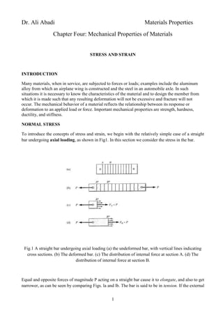
1. 1
Dr. Ali Abadi Materials Properties
Chapter Four: Mechanical Properties of Materials
STRESS AND STRAIN
INTRODUCTION
Many materials, when in service, are subjected to forces or loads; examples include the aluminum
alloy from which an airplane wing is constructed and the steel in an automobile axle. In such
situations it is necessary to know the characteristics of the material and to design the member from
which it is made such that any resulting deformation will not be excessive and fracture will not
occur. The mechanical behavior of a material reflects the relationship between its response or
deformation to an applied load or force. Important mechanical properties are strength, hardness,
ductility, and stiffness.
NORMAL STRESS
To introduce the concepts of stress and strain, we begin with the relatively simple case of a straight
bar undergoing axial loading, as shown in Fig1. In this section we consider the stress in the bar.
Fig.1 A straight bar undergoing axial loading (a) the undeformed bar, with vertical lines indicating
cross sections. (b) The deformed bar. (c) The distribution of internal force at section A. (d) The
distribution of internal force at section B.
Equal and opposite forces of magnitude P acting on a straight bar cause it to elongate, and also to get
narrower, as can be seen by comparing Figs. la and lb. The bar is said to be in tension. If the external

2. 2
forces had been applied in the opposite sense, that is, pointing toward each other, the bar would have
shortened and would then be said to be in compression.
Definition of Normal Stress: The thin arrows in Figs. 1c and ld represent the distribution of force on
cross sections at A and B, respectively. (A cross section is a plane that is perpendicular to the axis of
the bar.) Near the ends of the bar, for example at section A, the resultant normal force, FA, is not
uniformly distributed over the cross section; but at section B, farther from the point of application of
force P, the force distribution is uniform. In mechanics, the term stress is used to describe the
distribution of a force over the area on which it acts and is expressed as force intensity, that is, as
force per unit area.
Aera
Force
Stress 
The units of stress are units of force divided by units of area. In the International System of units
(SI), stress is specified using the basic units of force (Newton) and length (meter) as Newtons per
meter squared (N/m2
). This unit, called the Pascal (1 Pa = 1 N/m2
), is quite small, so in engineering
work stress is normally expressed in kilopascals (1 kPa = 103
N/m2
), megapascals (1 MPa = 106
N/m2
), or gigapascals (1 GPa = 109
N/m2
). For example,1 psi = 6895 Pa = 6.895 kPa. . In the U.S.
Customary System of units (USCS), stress is normally expressed in pounds per square inch (psi) or
in kips per square inch, that is, kilopounds per square inch (Ksi).
There are two types of stress, called normal stress and shear stress. In this section we will consider
only normal stress. In words, normal stress is defined by
actsforcethewhichonAera
areaantolarperpendicueinormalForce
stressNormal
.....
..).,.(

The symbol used for normal stress is the lowercase Greek letter sigma (σ). The normal stress at a
point is defined by the equation
)(lim),,(
0 A
F
zyx
A 



 Normal stress ………(1)
Where, as shown in Fig..2a, ΔF is the normal force (assumed positive in tension) acting on an
elemental area ΔA containing the point (x, y, z) where the stress is to be determined.

3. 3
Fig. 2 Normal force on a cross section
The sign convention for normal stress is as follows:
 A positive value for σ indicates tensile stress, that is, the stress due to a force ΔF that pulls
on the area on which it acts.
 A negative value for σ indicates compressive stress.
Average Normal Stress: Even when the normal stress varies over a cross section, as it does in Fig.
1c, we can compute the average normal stress on the cross section by letting
A
F
avg  Average Normal Stress ……(2)
Thus, for Figs. 1c and ld we get
A
P
A
FA
Aavg )( ,
A
P
A
FB
Bavg )(
Much of the rest of on going discussion is devoted to determining how stress is distributed on cross
sections of structural members under various loading conditions. However, in many situations the
normal stress on a cross section is either constant or very nearly constant, as we will see in the next
examples.
Prob. 1. A l-in.-diameter solid bar (1), a square solid bar (2), and a circular tubular member
with 0.2-in. wall thickness (3), each supports an axial tensile load of 5 kips, (a) Determine the

4. 4
axial stress in bar (1). (b) If the axial stress in each of the other bars is 6 ksi, what is the
dimension, b, of the square bar, and what is the outer diameter, c, of the tubular member?
P-1
Solution
(a) Axial stress
FBD: cylindrical solid bar
A
T
σ
1 in
X
Y
Definition:
ksi
in
kips
A
T
366.6
7854.0
5
2
1
1 
2
2
1
1 7854.0
4
)1(
4
in
ind
A 

σ1=6.37ksi
(b) Dimensions
FBD: square solid bar

5. 5
Prob. 2. The structural tee is shown in Fig. P-2 supports a compressive load P = 200 kN. (a)
Determine the coordinate yR of the point R in the cross section where the load must act in order to
produce uniform compressive axial stress in the member, and (b) determine the magnitude of that
compressive stress.
Definition: normal stress
.6
2
2 ksi
A
T
 2
2
2 bA 
in
T
b 9129.0
2


Definition: normal stress
)16.08.0(
46
5
526.1
8.0/]16.0)
4
([
)16.08.0(
4
])4.0([
4
3
3
3
22
3
3
3






c
ksi
kipsT
whereA
in
T
c
c
ccA
T







σ2
b T
b
A2
Y
X
cσ3
T
0.2 in
B=0.91 in
C=1.526 in

6. 6
P-2
)16.08.0(
46
5
526.1
8.0/]16.0)
4
([
)16.08.0(
4
])4.0([
4
3
3
3
22
3
3
3






c
ksi
kipsT
whereA
in
T
c
c
ccA
T








7. 7
Stress Resultant: Internal resultants were introduced in previous section, and Examples show how
equilibrium is used to relate these resultants on a cross section to the external loads. Equation 2
relates the average normal stress on a cross section to the normal force on the cross section. Let us
now examine in greater detail the relationship between the distributed normal stress on a cross
section and its resultant. Based on the definition of normal stress in Eq. 1, we can replace the ΔF in
Fig. 2a by an elemental force dF =σ dA. Referring again to Fig. 2a and following the right-hand rule
for moments, we can see that this elemental force dF contributes a moment zdF about the +y axis and
ydF about the -z axis. In Fig. 2b, the resultant normal force on the cross section at x is labeled F(x),
6.5mm
75mm 75mm
C1 .
6.5mm
y
C.
4mm
4mm
y 2=60mm
60mm
σ
P
Solution:
(a) point for uniform stress
Component(1)
Component (2):
(b) stress magnitude
FBD:
If P is applied at the cross-sectional centriod,
then the resulting axial stress will be uniform.
Therefore, R is the centroid.
component
y i
mm
Ai
mm2
y i Ai
mm3
1 126.5 1950 246675
2 60 960 57600
Sum Σ 2910 304275
Centroid of cross sectional area
mm
A
Ay
y
i
ii
R 56.104



yR = 105 mm
Definition: normal stress
A
P
 , iAA 
= 68.73 Mpa ( C )
σ =68.7 Mpa ( C )

8. 8
and it acts at point (yR, zR) in the cross section. Given the distribution of normal stress on a cross
section, σ = σ(x, y, z), we can integrate over the cross section to determine the magnitude and point
of application of the resultant normal force
:xF 
A
dAxF )(
:yM 
A
R dAzxFz )( …………… (3)
:zM 
A
R dAyxFy )(
The two moment equations are used to locate the line of action of the force F(x). Note that the sign
convention for or implies that the force F in Eq. 3 is to be taken positive in tension.
Resultant of Constant Normal Stress on a Cross Section: Let us determine the resultant of normal
stress on the cross section at x (Fig. 2a) if the normal stress is constant over the cross section. We
will prove that normal stress that is constant on a cross section corresponds to an axial force
F(x) = A σ (x) acting through the centroid of the cross section at x. (you will learn the conditions
under which σ (x) is constant over the cross section in later section.)
Let the resultant be assumed to be a force F(x) acting parallel to the x axis and passing through point
(yR, zR), as in Fig. 2b. We must show that
F(x) = A(x) σ (x),

 yyR ,

 zzR
For this we can use Eqs. 3. Substituting the condition σ (x, y, z) = σ (x) into Eqs. 3, we get
:xF AxdAxxF
A
)()()(   
:yM AzxzdAxxFz
A
R

  )()()( 
:zM AyxydAxxFy
A
R

  )()()( 
Therefore, if the normal stress is uniform over a cross section, the normal stress over the cross
section, also called the axial stress, and is given by

9. 9
)(
)(
)(
xA
xF
x  Axial Stress Equation …..(4)
Which corresponds to a force F(x) (tension positive) acting at the centroid of the cross section, that
is, at

 zzR ,

 yyR .
Uniform Normal Stress in an Axially Loaded Bar: tender certain assumptions, an axially loaded bar
will have the same uniform normal stress on every cross section; that is, σr (x, y, z) = σ = constant.
These assumptions are:
 The bar is prismatic; that is, the bar is straight and it has the same cross section throughout its
length.
 The bar is homogeneous; that is, the bar is made of the same material throughout.
 The load is applied as equal and opposite uniform stress distributions over the two end cross
sections of the bar.
The uniform, prismatic bar in Fig. 3a is labeled as member ―i‖ and is subjected to equal and opposite
axial forces Ft acting through the centroids at its ends. Its cross-sectional area is Ai.
Figure 3 Uniform stress in an axially loaded prismatic bar.
The normal stress on cross sections of an axially loaded member, like the one in Fig. 3, is called the
axial stress. Since, from the free-body diagram in Fig. 3b, the resultant force, F(x), on every cross
section of the bar is equal to the applied load Fi, and since the cross-sectional area is constant, from
Eq. 4 we get the fllowing formula for the uniform axial stress:
.const
A
F
i
i
i  Axial stress Equation (5)
Prob. 3. The diameter of the central one-third of a 50mm-diameter steel rod is reduced to 20
mm, forming a three segment rod, as shown in Fig. P-3. For the loading shown, Determine the
axial stresses (σ1, σ2 and σ3 in each of the three respective segments.

10. 10
P-3
p-4
Solution
Determine axial stress σ1, σ2, and σ3.
Equilibrium for FBD1:
:0 F -F1-20kN+20kN-10kN=0 F1=-10kN
Equilibrium for FBD2
:0 F -F2+20kN-10kN=0 F2=10kN
Equilibrium for FBD2
:0 F -F3-10kN=0 F3 = -10kN
Stresses:
iF

2
id
A

 2
F1 (1)
20kN 20kN 10kN
(2)F2
20kN
10kN
(3)
10kNF3

11. 11
Prob. 4. The three-part axially loaded member in Fig.P- 4 consists of a tubular segment (1)
with outer diameter (do)1=1.25 in. and inner diameter (di)1= 0.875 in., a solid circular rod
segment (2) with diameter d2 = 1.25 in., and another solid circular rod segment (3) with
diameter d3 = 0.875 in. The line of action of each of the three applied loads is along the
centroidal axis of the member. Determine the axial stresses σ1, σ2, and σ3 in each of the three
respective segments.
FBD: section (1), (2) and (3)
FBD: section (2) +(3)
FBD: section (3)
F1 (1) (2) (3)
0.875 in
1.25 in
3 kips 4kips 2kips
0.875 in
F2
1.25 in (2) (1) 2 kips
4 kips
F3
0.875in 2kips
(3)
y
x
σ1= 4.79ksi
σ2=4.89ksi
σ3=3.336ksi
Equilibrium
:0 xF
-F1 -3kips +4kips +2kips= 0
F1= 3kips
])875.0()25.1[(
4
22
1 ininA 

ksi
A
F
793.4
1
1
1 
Equilibrium
:0 xF
-F2+4kips +2kips= 0, F2 =6kips
2
2 )25.1(
4
inA


ksi
A
F
889.4
2
2
2 
Equilibrium
:0 xF
-F3+2kips= 0, F3 =2kips
2
3 )875.0(
4
inA


ksi
A
F
326.3
3
3
3 

12. 12
Engineering strain:
Engineering strain is defined according to
∈=
𝑙 𝑖− 𝑙 𝑜
𝑙 𝑜
…………………….. (6)
in which lo is the original length before any load is applied, and li is the instantaneous length.
Sometimes the quantity li – lo is denoted as ∆𝑙 and is the deformation elongation or change in length
at some instant, as referenced to the original length. Engineering strain (subsequently called just
strain) is unitless. Sometimes strain is also expressed as a percentage, in which the strain value is
multiplied by 100.
Compression Tests:
A compression test is conducted in a manner similar to the tensile test, except that the force is
compressive and the specimen contracts along the direction of the stress. Equations 5 and 6 are
utilized to compute compressive stress and strain, respectively. By convention, a compressive force
is taken to be negative, which yields a negative stress. The strain is positive if the materials are
stretched or negative if they are compressed.
Tensile tests are more common because they are easier to perform; also, for most materials used in
structural applications, very little additional information is obtained from compressive tests.
Compressive tests are used when the material is brittle in tension.
Shear and Torsional Tests:
For tests performed using a pure shear force as shown in Figure below, the shear stress is computed
according to
𝜏 =
𝐹
𝐴 𝑂
……………… (7)
Where F is the load or force imposed parallel to the upper and lower faces, each of which has an area
of Ao. The shear strain γ is defined as the tangent of the strain angle , as indicated in the figure. The
unit for shear stress is Pascal.
Torsion is a variation of pure shear, wherein a structural member is twisted in the manner of Figure
below; torsional forces produce a rotational motion about the longitudinal axis of one end of the
member relative to the other end. Examples of torsion are found for machine axles and drive shafts,
and also for twist drills. Torsional tests are normally performed on cylindrical solid shafts or tubes. A
shear stress is a function of the applied torque T, whereas shear strain is related to the angle of twist,
in Figure below.

13. 13
Geometric Considerations of the Stress State:
Consider the cylindrical tensile specimen of Figure below that is subjected to a tensile stress σ
applied parallel to its axis. Furthermore, consider also the plane 𝑝 − 𝑝,
that is oriented at some
arbitrary angle relative to the plane of the specimen end-face. Upon this plane 𝑝 − 𝑝,
, the applied
stress is no longer a pure tensile one. Rather, a more complex stress state is present that consists of a
tensile (or normal) stress 𝜍,
that acts normal to the 𝑝 − 𝑝,
plane and, in addition, a shear stress 𝜏,
that
acts parallel to this plane; both of these stresses are represented in the figure below. Using mechanics
of materials principles, it is possible to develop equations for 𝜍,
and 𝜏,
in terms of σ and θ, as
follows:
𝜍,
= 𝜍𝑐𝑜𝑠2
𝜃 = 𝜍
1+cos 2𝜃
2
………… (8 a)
𝜏,
= 𝜍 sin 𝜃 cos 𝜃 = 𝜍
𝑠𝑖𝑛2𝜃
2
………. (8 b)
Figure Schematic representation showing normal ( 𝜍,
)
and shear ( 𝜏,
) stresses that act on a plane oriented at an
angle θ relative to the plane taken perpendicular to the
direction along which a pure tensile stress (σ) is applied.

14. 14
Elastic Deformation
Stress-Strain Behavior
The degree to which a structure deforms or strains depends on the magnitude of an imposed stress.
For most metals that are stressed in tension and at relatively low levels, stress and strain are
proportional to each other through the relationship:
𝝈 = 𝑬 ∈ ………………….. (9) [Hooke’s law— relationship between engineering stress and engineering
strain for elastic deformation (tension and compression)]
Note: Hooke’s Law describes only the initial linear portion of the stress-strain curve for a bar
subjected to uniaxial extension.
The constant of proportionality E (GPa or psi), The slope of the straight-line portion of the stress-
strain diagram is called the Modulus of Elasticity or Young’s Modulus.
The SI unit for the modulus of elasticity is gigapascal, GPa, where 1 GPa N/m2
= 103
MPa. The
moduli of elasticity are slightly higher for ceramic materials, Polymers have modulus values that are
smaller than both metals and ceramics.
Room temperature modulus of elasticity values for a number of metals, ceramics, and polymers are
presented in Table below.
A plot of stress (ordinate) versus strain (abscissa) results in a linear relationship, as shown in Figure
below. Elastic deformation is nonpermanent, which means that when the applied load is released, the
piece returns to its original shape. As shown in the stress–strain plot.
Schematic stress–strain diagram showing linear elastic
deformation for loading and unloading cycles.
There are some materials (e.g., gray cast iron, concrete, and many polymers) for which this elastic
portion of the stress–strain curve is not linear (Figure below); hence, it is not possible to determine a
modulus of elasticity as described above. For this nonlinear behavior, either tangent or secant
modulus is normally used. Tangent modulus is taken as the slope of the stress–strain curve at some
specified level of stress, while secant modulus represents the slope of a secant drawn from the
origin to some given point of the stress– strain curve. The determination of these moduli is illustrated
in Figure below

15. 15
.
Schematic stress–strain
diagram showing non-linear
elastic behavior, and how
secant and tangent moduli are
determined.
The stress–strain characteristics at low stress levels are virtually the same for both tensile and
compressive situations, to include the magnitude of the modulus of elasticity. Shear stress and strain
are proportional to each other through the expression
(
G = τ/γ (shear stress – strain) [Relationship between shear stress and shear strain for elastic deformation]
Where G is the shear modulus or Modulus of Rigidity, the slope of the linear elastic r
egion of the shear stress–strain curve.
Anelasticity:
So far we have assumed that elastic deformation is time independent (i.e. applied stress produces
instantaneous elastic strain)
However, in reality elastic deformation takes time (finite rate of atomic/molecular deformation
processes) - continues after initial loading, and after load release. This time dependent elastic
behavior is known as anelasticity.
The effect is normally small for metals but can be significant for polymers (―visco-elastic behavior‖).

16. 16
Example: Elongation (Elastic) Computation
A piece of copper originally 305 mm (12 in.) long is pulled in tension with a stress of 276 MPa
(40,000 psi). The magnitude of E for copper is 110 GPa (16X106
psi). If the deformation is
entirely elastic, what will be the resultant elongation?
Elastic Deformation: Poisson’s ratio
When a tensile stress is imposed on a metal specimen, an elastic elongation and accompanying
strain𝜖 𝑧 result in the direction of the applied stress (arbitrarily taken to be the z direction), as
indicated in Figure below. As a result of this elongation, there will be constrictions in the lateral (x
and y) directions perpendicular to the applied stress. If the applied stress is uniaxial (only in the z
direction), and the material is isotropic, then𝜖 𝑥 = 𝜖 𝑦 . A parameter termed Poisson’s ratio (ν) is
defined as the ratio of the lateral and axial strains, or
= lateral/axial
𝜐 = −
𝜖 𝑥
𝜖 𝑧
= −
𝜖 𝑦
𝜖 𝑧
………….. (10)
υ is dimensionless .The negative sign is included in the expression so that will always be positive,
since 𝜖 𝑥 and 𝜖 𝑧will always be of opposite sign or (sign shows that lateral strain is in opposite sense to
longitudinal strain). Theoretically, Poisson’s ratio for isotropic materials should be 0.25 and
maximum value: 0.50, Typical value: 0.24 - 0.30.

17. 17
For isotropic materials, shear and elastic moduli are related to each other and to Poisson’s ratio
according to
E = 2G (1+υ) → In most metals G ~ 0.4E
G is Shear Modulus (Units: N/m2
)
(Note: most materials are elastically anisotropic: the elastic behavior varies with crystallographic
direction)
For these materials the elastic properties are completely characterized only by the specification of
several elastic constants, their number depending on characteristics of the crystal structure. Even for
isotropic materials, for complete characterization of the elastic properties, at least two constants must
be given. Since the grain orientation is random in most polycrystalline materials, these may be
considered to be isotropic; inorganic ceramic glasses are also isotropic. The remaining discussion of
mechanical behavior assumes isotropy and polycrystallinity because such is the character of
most engineering materials.
Example: Computation of Load to Produce Specified Diameter Change
A tensile stress is to be applied along the long axis of a cylindrical brass rod that has a diameter
of 10 mm (0.4 in.). Determine the magnitude of the load required to produce a 2.5x10-3
mm (
10-4
in.) change in diameter if the deformation is entirely elastic. The value for Poisson’s ratio
for brass is 0.34
When the force F is applied, the specimen will
elongate in the z direction and at the same time
experience a reduction in diameter,Δd of 2.5x10-3
mm in the x direction. For the strain in the x
direction,
Which is negative, since the diameter is reduced

18. 18
Plastic deformation:
• Stress and strain are not proportional
• The deformation is not reversible
• Deformation occurs by breaking and re-arrangement of atomic bonds (in crystalline materials
primarily by motion of dislocations)
Yield strength σy - is chosen as that causing a
permanent strain of 0.002
Yield point P - the strain deviates from being
proportional to the stress (the proportional limit)
The yield stress is a measure of resistance to
plastic deformation

19. 19
And in more details we can classify a stress as shown in figure below.
σPL ( Proportional Limit) - Stress above which stress is not longer proportional to strain.
σEL ( Elastic Limit) - The maximum stress that can be applied without resulting in permanent
deformation when unloaded.
σYP ( Yield Point) - Stress at which there are large increases in strain with little or no increase in
stress. Among common structural materials, only steel exhibits this type of response.
σYS ( Yield Strength) - The maximum stress that can be applied without exceeding a specified value
of permanent strain (typically .2% = .002 in/in).
σU ( Ultimate Strength) - The maximum stress the material can withstand (based on the original
area).
Tensile Properties:
A typical stress-strain curve is shown in Figure below. If we begin from the origin and follow the
graph numbers of points are indicated.

20. 20
Point A: At origin, there is no initial stress or strain in the test piece. Up to point A Hooke's Law is
obeyed according to which stress is directly proportional to strain. That's why the point A is also
known as proportional limit. This straight line region is known as elastic region and the material can
regain its original shape after removal of load.
Point B: The portion of the curve between AB is not a straight line and strain increases faster than
stress at all points on the curve beyond point A. Point B is the point after which any continuous stress
results in permanent, or inelastic deformation. Thus, point B is known as the elastic limit or yield
point.
Point C & D: Beyond the point B, the material goes to the plastic stage till the point C is reached. At
this point the cross- sectional area of the material starts decreasing and the stress decreases to point
D. At point D the workpiece changes its length with a little or without any increase in stress up to
point E.
Point E: Point E indicates the location of the value of the ultimate stress. The portion DE is called
the yielding of the material at constant stress. From point E onwards, the strength of the material
increases and requires more stress for deformation, until point F is reached. The tensile strength
(MPa or psi) is the stress at the maximum on the engineering stress–strain curve.
Point F: A material is considered to have completely failed once it reaches the ultimate stress. The
point of fracture, or the actual tearing of the material, does not occur until point F. The point F is also
called ultimate point or fracture point.
Example: Mechanical Property Determinations from Stress–Strain Plot
From the tensile stress–strain behavior for the brass specimen shown in
Figure below, determine the following:
(a) The modulus of elasticity
(b) The yield strength at a strain offset of 0.002
(c) The maximum load that can be sustained by a cylindrical specimen having an original
diameter of 12.8 mm (0.505 in.)
(d) The change in length of a specimen originally 250 mm (10 in.) long that is subjected to a
tensile stress of 345 MPa (50,000 psi)
Solution
(a) The modulus of elasticity is the slope of the elastic or initial linear portion of the stress–strain
curve. The strain axis has been expanded in the inset, Figure below, to facilitate this
computation. The slope of this linear region is the rise over the run, or the change in stress
divided by the corresponding change in strain; in mathematical terms,
E=slope =
∆𝜍
∆𝜖
=
𝜍2−𝜍1
𝜖2−𝜖1

21. 21
Inasmuch as the line segment passes through the origin, it is convenient to take both 𝜍1 and 𝜖1 as
zero. If 𝜍2 is arbitrarily taken as 150 MPa, then 𝜖2 will have a value of 0.0016. Therefore,
𝐸 =
150−0 𝑀𝑃𝑎
0.0016−0
= 93.8 𝐺𝑃𝑎 (13.6 x 106
psi)
which is very close to the value of 97 GPa ( psi) given for brass in tables.
(b) : The 0.002 strain offset line is constructed as shown in the inset; its intersection with the stress–
strain curve is at approximately 250 MPa (36,000 psi), which is the yield strength of the brass.
(c) : The maximum load that can be sustained by the specimen is calculated by using Equation 6.1, in
which σ is taken to be the tensile strength, from the above Figure, 450 MPa (65,000 psi). Solving for
F, the maximum load, yields
𝐹 = 𝜍𝐴 𝑂 = 𝜍
𝑑 𝑜
2
2
𝜋
𝐹 = 450𝑥106 𝑁
𝑚2
12.8𝑥10−3 𝑚
2
2
π = 57.9 N (13 Ibf)
(d) : To compute the change in length, ΔL, it is first necessary to determine the strain that is
produced by a stress of 345 MPa. This is accomplished by locating the stress point on the stress–
strain curve, point A, and reading the corresponding strain from the strain axis, which is
approximately 0.06.
Inasmuch as lo = 250 mm, we have
∆𝑙 = 𝜖𝑙 𝑜= (0.06)(250 mm)= 15 mm (0.6 in.)

22. 22
Ductility:
Ductility is another important mechanical property. It is a measure of the degree of plastic
deformation at fracture. A material that experiences very little or no plastic deformation upon
fracture is termed brittle. The tensile stress–strain behaviors for both ductile and brittle materials are
schematically illustrated in Figure below.
Ductility may be expressed quantitatively as
either percent elongation or percent
reduction in area. The percent elongation
%EL is the percentage of plastic strain at
fracture, or
% EL=
𝑙 𝑓−𝑙 𝑜
𝑙0
x 100 or
%EL = max x 100 %
Where 𝑙𝑓 is the fracture length and 𝑙 𝑜 is the
original gauge length
Ductility defined by percent reduction in area
%RA=
𝐴 𝑂 −𝐴 𝑓
𝐴0
𝑋 100
Where 𝐴 𝑂 is the original cross-sectional area and 𝐴𝑓 is the cross-sectional area at the point of
fracture. Both 𝑙𝑓 and𝐴𝑓 are measured subsequent to fracture and after the two broken ends have
been repositioned back together.
 Percent reduction in area values are independent of both 𝑙 𝑜and 𝐴 𝑂
 Most metals possess at least a moderate degree of ductility at room temperature;
 some become brittle as the temperature is lowered.
 Knowledge of the ductility of materials is important for at least two reasons.
 First, it indicates to a designer the degree to which a structure will deform plastically
before fracture.
 Second, it specifies the degree of allowable deformation during fabrication operations
 Brittle materials are approximately considered to be those having a fracture strain of less than
about 5%.
 Table below presents some typical values of mechanical properties of several metals and
alloys at room-temperature.
 The yield strength and tensile strength vary with prior thermal and mechanical treatment,
impurity levels, etc. This variability is related to the behavior of dislocations in the material.
 But elastic moduli are relatively insensitive to these effects.
 The yield and tensile strengths and modulus of elasticity decrease with increasing
temperature.
 Ductility increases with temperature.

23. 23
Resilience:
Is the capacity of a material to absorb energy when it is deformed elastically and then, upon
unloading, to have this energy recovered.
Modulus of resilience (Ur): This is the strain energy per unit volume required to stress a material
from an unloaded state up to the point of yielding. (Area under the elastic line)
𝑈𝑟 = 𝜍𝑑𝜖
𝜖 𝑦
0
Ur = ½ σy εy
Assuming a linear elastic region,
𝑈𝑟 =
1
2
𝜍𝑦 𝜖 𝑦
From Hooks law
𝜖 𝑦 = 𝜍
𝐸
𝑈𝑟 =
𝜍𝑦
2
2𝐸
(units should represent energy: Joule/m3
)
Units: MPa= N/m2
x 106
N/m2
x m/m =J/m3
Thus, resilient materials are those having high yield strengths and low moduli of elasticity; such
alloys would be used in spring applications.

24. 24
Toughness:
Is a measure of the ability of a material to absorb energy up to fracture.
An approximation for the Ut is the area under the
curve. Where Ut is a modulus of toughness
It depends on both strength and ductility of
the material in question. A neighbor figure
is given to show the relationship between the
stress and strain for three materials.
From the figure, it can be concluded that
tensile toughness is the area under the stress
- strain curve. It is high if a material has
high amount of strength and ductility.
Materials with low ductility of low strength
don't posses ample tensile toughness.
The word toughness is usually used for tensile toughness. In tensile toughness, the strain rate is
relatively slow.

25. 25
True stress and strain:
σT= F / Ai , load divided by the instantaneous cross section area
εT= ln(li/ lo), li: instantaneous length , lo: original length
For plastic deformation (σ>σy) there is conservation of
volume: Aolo= Aili Ao/ Ai = li/lo
Relations between true and engineering stress and strain:
σT= F / Ai = F / Ao x Ao/ Ai= σ x Ao/Ai = σ x li / lo
ε= li-lo / lo = li/lo –1
li/lo = 1+ ε
Thus σT= σ(1+ ε)This equation is valid from yielding to the on set of necking σy< σ < σu

T= ln (li/ lo) = ln(1+ε), This equation is valid from yielding to the on set of necking σy< σ < σu
For some metals and alloys the region of the true stress –strain curve from the onset of plastic
deformation to the point at which necking begins (σy< σ < σu) may be approximated by:
𝜍 𝑇 = 𝐾 𝜖 𝑇
𝑛
n is hardening exponent = 0.15 for some steels
= 0.5 for some copper
𝜖 𝑇 is true strain: ln(li /lo)
𝜍 𝑇is true stress (F / A)
𝐾 is a strength coefficient
K and n are constants that vary from alloy to alloy. and will also depend on the condition of the
material (i.e., whether it has been plastically deformed, heat treated, etc.). The parameter n is often
has a value less than unity
Taking logarithm of both sides yields a straight line:

26. 26
Log σT= n log εT+ log K
(y=mx+c)
n (strain hardening exponent) defines the slope of the straight line
Example:
Example:

27. 27
Example:
For a brass alloy, the following engineering stresses produce the corresponding plastic engineering
strain, prior to necking:
Engineering Stress (MPa) Engineering Strain
315 0.105
340 0.220
On the basis of this information, compute the engineering stress necessary to produce an engineering
strain of 0.28.

28. 28
Hardness:
Hardness is a measure of the material’s resistance to localized plastic deformation (e.g. dent or
scratch) A qualitative Moh’s scale, determined by the ability of a material to scratch another
material: from 1 (softest = talc) to 10 (hardest = diamond).
Diamond 10
Corundum 9
Topaz 8
Quartz 7
Orthoclase (Feldspar) 6
Apatite 5
Fluorite 4
Calcite 3
Gypsum 2
Talc 1
Different types of quantitative hardness test have been designed (Rockwell, Brinell, Vickers, etc.).
Usually a small indenter (sphere, cone, or pyramid) is forced into the surface of a material under
conditions of controlled magnitude and rate of loading. The depth or size of indentation is measured.
The tests somewhat approximate, but popular because they are easy and non-destructive (except for
the small dent).

29. 29
Quantitative hardness techniques have been developed over the years in which a small indenter is
forced into the surface of a material to be tested, under controlled conditions of load and rate of
application. The depth or size of the resulting indentation is measured, which in turn is related to a
hardness number; the softer the material, the larger and deeper is the indentation, and the lower the
hardness index number.
Hardness tests are performed more frequently than any other mechanical test for several reasons:
1. They are simple and inexpensive—ordinarily no special specimen need be prepared, and the
testing apparatus is relatively inexpensive.
2. The test is nondestructive—the specimen is neither fractured nor excessively deformed; a small
indentation is the only deformation.
3. Other mechanical properties often may be estimated from hardness data, such as tensile strength
Rockwell Hardness Test:
Stanley P. Rockwell invented the Rockwell hardness test. He was a metallurgist for a large ball
bearing company and he wanted a fast non-destructive way to determine if the heat treatment process
they were doing on the bearing races was successful. The only hardness tests he had available at time
were Vickers, Brinell and Scleroscope. The Vickers test was too time consuming, Brinell indents
were too big for his parts and the Scleroscope was difficult to use, especially on his small parts.
To satisfy his needs he invented the Rockwell test method. This simple sequence of test force
application proved to be a major advance in the world of hardness testing. It enabled the user to
perform an accurate hardness test on a variety of sized parts in just a few seconds.
The Rockwell tests constitute the most common method used to measure hardness and generally
accepted due to
1) Its speed
2) Freedom from personal error (require no special skills).
3) Ability to distinguish small hardnessdifference
4) Small size of indentation.
5) They are so simple to perform.
The Rockwell hardness test method consists of indenting the test material with a diamond cone or
hardened steel ball indenter. The indenter is forced into the test material under a preliminary minor
load F0 (Fig. A) usually 10 kgf. When equilibrium has been reached, an indicating device, which
follows the movements of the indenter and so responds to changes in depth of penetration of the
indenter is set to a datum position. While the preliminary minor load is still applied an additional
major load is applied with resulting increase in penetration (Fig. B). When equilibrium has again
been reach, the additional major load is removed but the preliminary minor load is still maintained.
Removal of the additional major load allows a partial recovery, so reducing the depth of penetration
(Fig. C), (The hardness is measured according to the depth of indentation, under a constant load).
The permanent increase in depth of penetration, resulting from the application and removal of the
additional major load is used to calculate the Rockwell hardness number.
HR = E - e
F0 = preliminary minor load in kgf
F1 = additional major load in kgf
F = total load in kgf
e = permanent increase in depth of penetration due to major load F1 measured in units of 0.002 mm
E = a constant depending on form of indenter: 100 units for diamond indenter, 130 units for steel ball
indenter

30. 30
HR = Rockwell hardness number
D = diameter of steel ball
Rockwell Principle
Principal of the Rockwell Test:
• Position the surface area to be measured close to the indenter.
• Applied the minor load and a zero reference position is established
• The major load is applied for a specified time period (dwell time) beyond zero
• The major load is released leaving the minor load applied.
 The Rockwell number represents the difference in depth from the zero reference position as
a result of the applied major load.
 Deeper indentation means softer material
Types of the Rockwell Test:
There are two types of Rockwell tests:
1. Rockwell: the minor load is 10 kgf, the major load is 60, 100, or 150 kgf.
2. Superficial Rockwell: the minor load is 3 kgf and major loads are 15, 30, or 45 kgf.
In both tests, the indenter may be either a diamond cone or steel ball, depending upon the
characteristics of the material being tested.

31. 31
Rockwell hardness scale:
Rockwell hardness values are expressed as a combination of a hardness number and a scale symbol
representing the indenter and the minor and major loads. The hardness number is expressed by the
symbol HR and the scale designation.
There are 30 different scales. The majority of applications are covered by the Rockwell C and B
scales for testing steel, brass, and other metals. However, the increasing use of materials other than
steel and brass as well as thin materials necessitates a basic knowledge of the factors that must be
considered in choosing the correct scale to ensure an accurate Rockwell test. The choice is not only
between the regular hardness test and superficial hardness test, with three different major loads for
each, but also between the diamond indenter and the 1/16, 1/8, 1/4 and 1/2 in. diameter steel ball
indenters.
If no specification exists or there is doubt about the suitability of the specified scale, an analysis
should be made of the following factors that control scale selection:
 Type of material
 Specimen thickness
 Test location
 Scale limitations
• The Hardened steel is tested on the C scale with Rc20-70.
• Softer materials are tested on the B scale with Rb30-100.
Brale indenter,120o
diamond cone
1.6-3.2 mm diameter steel ball indenter
On the basis of the magnitude of both major and minor loads, there are two types of tests:
 Rockwell and superficial Rockwell. For Rockwell, the minor load is 10 kg, whereas major
loads are 60, 100, and 150 kg.
 Each scale is represented by a letter of the alphabet;
 For superficial tests, 3 kg is the minor load; 15, 30, and 45 kg are the possible major load
values.
 These scales are identified by a 15, 30, or 45 (according to load), followed by N, T,W, X, or
Y, depending on indenter.
 Superficial tests are frequently performed on thin specimens.

32. 32
Table of Rockwell Hardness Scales:
Scale Indenter
Minor Load
F0(kgf)
Major Load
F1(kgf)
Total Load
F(kgf)
Value of
E
A Diamond cone 10 50 60 100
B 1/16" steel ball 10 90 100 130
C Diamond cone 10 140 150 100
D Diamond cone 10 90 100 100
E 1/8" steel ball 10 90 100 130
F 1/16" steel ball 10 50 60 130
G 1/16" steel ball 10 140 150 130
H 1/8" steel ball 10 50 60 130
K 1/8" steel ball 10 140 150 130
L 1/4" steel ball 10 50 60 130
M 1/4" steel ball 10 90 100 130
P 1/4" steel ball 10 140 150 130
R 1/2" steel ball 10 50 60 130
S 1/2" steel ball 10 90 100 130
V 1/2" steel ball 10 140 150 130
Superficial Rockwell Hardness Scales
Scale Indenter Type
Minor Load
F0(kgf)
Major Load
F1(kgf)
Total Load
F(kgf)
Value of
E
HR 15 N N Diamond cone 3 12 15 100
HR 30 N N Diamond cone 3 27 30 100
HR 45 N N Diamond cone 3 42 45 100
HR 15 T 1/16" steel ball 3 12 15 100
HR 30 T 1/16" steel ball 3 27 30 100
HR 45 T 1/16" steel ball 3 42 45 100
HR 15 W 1/8" steel ball 3 12 15 100
HR 30 W 1/8" steel ball 3 27 30 100
HR 45 W 1/8" steel ball 3 42 45 100
HR 15 X 1/4" steel ball 3 12 15 100
HR 30 X 1/4" steel ball 3 27 30 100
HR 45 X 1/4" steel ball 3 42 45 100
HR 15 Y 1/2" steel ball 3 12 15 100
HR 30 Y 1/2" steel ball 3 27 30 100
HR 45 Y 1/2" steel ball 3 42 45 100

33. 33
The scale is designated by the symbol HRfollowed by the appropriate scale identification. For
example, 80 HRB represents a Rockwell hardness of 80 on the B scale, and 60 HR30W indicates a
superficial hardness of 60 on the 30W scale.
Scales properties:
i. All are dimensionless
ii. All have maximum reading of 130
iii. Become inaccurate below 20 or above 100
Rockwell Hardness Scales in brief:
a. Rockwell B: for unhardened carbon steels, copper, aluminum, malleable cast iron
i. 1/16" dia. steel ball
ii. 100 kg major load
iii. range: 0-100
b. Rockwell C: for steel, hardened steel, case hardened steel, pearlitic cast iron,
titanium, others w/RB > 100
i. 120° diamond cone (―Brale‖) indenter
ii. 150 kg load
iii. range: 20-70
c. Rockwell A: for thinner or more brittle specimens of the RC family of materials:
cemented carbides, thin case hardened parts, thin gauge steel
i. Brale indenter
ii. 60 kg load
iii. Extended useful range
d. Other standard tests: D, E, F, G, H, K, L, M, P, R, S, V
e. Superficial: N (Brale indenter), T (1/16" dia. steel ball), W(1/8" dia. steel ball), X, Y
i. Same indenters as standard tests
ii. 15, 30, or 45-kg major loads — e.g. 30N, 45T
Rockwell hardness instruction:
• Cleaned and well seated indenter and anvil.
• Surface which is clean and dry, smooth and free from oxide.
• Flat surface, which is perpendicular to the indenter.
• Cylindrical surface gives low readings, depending on the curvature.
• Thickness should be 10 times higher that the depth of the indenter.
• The spacing between the indentations should be 3 or 5 times the diameter of the indentation.
• Loading speed should be standardised.

34. 34
Brinell hardness:
J.A. Brinell introduced the first standardized indentation-hardness test in 1900. The Brinell hardness
test consists in indenting the metal surface with a 10-mm diameter steel or tungsten carbide ball at a
load range of 500-3000 kg, depending of hardness of particular materials.
The load is applied for a standard time ( between 10 - 30 s), and the diameter of the indentation is
measured. Giving an average value of two readings of the diameter of the indentation at right angle.
• The Brinell hardness number (BHN or HB) is expressed as
the load P divided by surface area of the indentation.
Where:
P: applied load (kgf)
D: diameter of ball (indenter) (mm)
d: diameter of indentation (mm)
The Brinell hardness number followed by the symbol HB
denotes standard test conditions of 3000 kg, 10mm ball and
10-15 seconds loading.
Other testing conditions are suffixed as 'ball/kgs/load duration
(secs)' after the number obtained and HB symbol (ie. 50.3 HB 10/500/30) for 10mm ball, 500 kg, 30
seconds load and an impression reading of 3.50mm.
Unit kgf.mm-2
=9.8 MPa
Advantage and disadvantages of Brinell hardness test
• Large indentation averages out local heterogeneities of microstructure.
• Different loads are used to cover a wide range of hardness of commercial metals.
• Brinell hardness test is less influenced by surface scratches and roughness than other hardness tests.
• The test has limitations on small specimens or in critically stressed parts where indentation could be
a possible site of failure

35. 35
Brinell hardness test with nonstandard load or ball diameter:
• From figure below, d = Dsinφ, giving the alternative expression of Brinell hardness number as
𝐵𝐻𝑁 =
𝑃
𝜋
2 𝐷2 1 − 𝐶𝑂𝑆𝜑
• In order to obtain the same BHN with a non-standard
load or ball diameter, it is necessary to produce a
geometrical similar indentations.
• The included angle 2φ should remain constant and the load and the ball diameter must be varied in
the ratio
𝑃1
𝐷1
2 =
𝑃2
𝐷2
2 =
𝑃3
𝐷3
2
Meyer hardness
• Meyer suggested that hardness should be expressed in terms of the mean pressure between the
surface of the indenter and the indentation, which is equal to the load divided by the projected area of
the indentation
• Meyer hardness is therefore expressed as follows;
Note: - Meyer hardness is less sensitive to the applied load than Brinell hardness.
- Meyer hardness is a more fundamental measure of indentation hardness but it is rarely used for
practical hardness measurement
Vickers hardness:
• Vickers hardness test uses a square-base diamond pyramid as the indenter with the included angle
between opposite faces of the pyramid of 136o
.
• The Vickers hardness number (VHN) is defined as the load divided by the surface area of the
indentation

36. 36
𝑉𝐻𝑁 =
2𝑃𝑠𝑖𝑛 𝜃
2
𝐿2
=
1.854𝑃
𝐿2
Where P is the applied load, kg
L is the average length of diagonals, mm
θ is the angle between opposite faces of diamond = 136o
.
Note: not widely used for routine check due to a slower process and requires careful surface
preparation.
Note: the unite can be VHN, DPH, Hv
•
Vickers hardness test uses the loads ranging from 1-120 kgf, applied for between 10 and 15
seconds.
• Provide a fairly wide acceptance for research work because it provides a continuous scale of
hardness, for a given load.
• VHN = 5-1,500 can be obtained at the same load level (easy for comparison).
Vickers hardness values of materials:
Materials Hv
Tin 5
Aluminum 25
Gold 35
Copper 40
Iron 80
Mild steel 230
Full hard steel 1000
Tungsten carbide 2500
Knoop hardness:
1. Microhardness only
2. Elongated diamond indenter
a. 172° 30' between long edges
b. 130° 0' between short edges
3. Useful for…
a. … surfaces
b. … elongated microconstituents
c. … anisotropic properties — only measure long dimension of indent, which can be reoriented
w.r.t. texture (of polycrystalline sample) or crystallographic axes (of a single-crystal sample)
3. Defined as load/projected area of indentation (in
contrast to Vickers)
5. KHN 
𝑃
𝐴 𝑃
=
𝑃
𝐶𝐿2
P: applied load, kg
L: length of long diagonal, mm
C: constant relating projected area to length of long diagonal, 0.07028 for dimensions given
Above
6. Applied loads are much smaller than for Rockwell and Brinell, ranging between 1 and 1000 g
7. Hardness scales for both techniques are approximately equivalent
8. Both are well suited for measuring the hardness of small, selected specimen regions
9. Knoop is used for testing brittle materials such as ceramics

37. 37
Vickers and Knoop:
1. Slow
2. Sensitive to surface condition
a. Requires polishing (through diamond or -Al2O3 step)
b. Best unetched
3. Requires load to be normal to surface plane parallel surfaces
4. Can be done on mounted specimens
5. Subject to error in diagonal measurement
6. Comparison
a. Knoop — shallower indent more surface sensitivity
b. Vickers — smaller L more prone to measurement errors
Shore Scleroscope Hardness Test:
 The Shore Scleroscope hardness is associated with the elasticity of the material.
 The appliance consists of a diamond-tipped hammer, which falls inside a graduated glass tube
with the numbers starting from the bottom upward, under the force of its own weight
(weighing less than an ounce) from a fixed height, onto the test specimen. The tube is divided
into 140 equal parts.
 The hammer is brought to the top of the tube by a vacuum, and then, being released, falls on
the part to be tested
 The height of the first rebound is the hardness index of the material.
 The harder the material, the higher the rebound.
 The Shore method is widely used for measuring hardness of large machine components like
rolls, gears, dies, etc.
 Advantages of this method are small, mobile and non-marking of the test surface.

38. 38
The Durometer:
 The Durometer is a popular instrument for measuring the indentation hardness of rubber and
rubber-like materials. The most popular testers are the Model A used for measuring softer
materials and the Model D for harder materials.
 The operation of the tester is quite simple. The material is subjected to a definite pressure
applied by a calibrated spring to an indenter that is either a cone or sphere and an indicating
device measures the depth of indentation.
Microhardness:
 Microhardness testing specifies an allowable range of loads for testing with a diamond
indenter.
 The resulting indentation is then recorded and converted to a hardness value. Typically loads
are very light, ranging from a few grams to one or several kilograms.
 Since the test indentation is very small, microhardness testing is useful for a variety of
applications such as testing very thin materials like foils or measuring individual
microstructures.
 The procedure for testing is very similar to that of the standard Vickers hardness test, except
that it is done on a microscopic scale with higher precision instruments.
 Precision microscopes are used to measure the indentations; these usually have a
magnification of around X500 and measure to an accuracy of +0.5 micrometers.
Correlation Between Hardness and Tensile Strength:
Both tensile strength and hardness are indicators of a metal’s resistance to plastic deformation.
Consequently, they are roughly proportional, as shown in Figure below, for tensile strength as a
function of the HB for cast iron, steel, and brass. The same proportionality relationship does not hold
for all metals, as Figure below indicates. As a rule of thumb for most steels, the HB and the tensile
strength are related according to:
TS(MPa) = 3.45x HB (For steel alloys, conversion of Brinell hardness to tensile strength)
TS(psi) = 500 x HB

39. 39
Both tensile strength and hardness may be regarded as degree of resistance to plastic deformation.
Hardness is proportional to the tensile strength – but note that the proportionality constant is different
for different materials.
Design stress: σd = N’σc
where σc = maximum anticipated stress, N’ is the ―design factor‖ > 1.
Want to make sure that σd < σy
Safe or working stress: σw = σy/N where N is ―factor of safety‖ > 1.
EXAMPLE 1-1
Consider the maximum load on the structure is known with an uncertainity of ± 20 %, the load
causing failure is known within ± 15 %. If the load causing failure is nominally 9 kN, determine the
design factor and the maximum allowable load that will ofset the absolute uncertainties.
Solution: To account for its uncertainity the loss of function load must increase to 1/0.85, whereas
the maximum allowable load must decrease to1/1.2. Thus to offset the absolute uncertainties the
design factor should be: 𝑛 𝑑 =
1
0.85
1
1.2
= 1.4

40. 40
Maximum allowable load=
9
14
= 6.4 kN
It is more common to express the design factor in terms of stress and a relevant strength. Thus:
nd =loss-of-function strength/allowable stress= 𝑆
𝜍
EXAMPLE 1-2
A rod with a cross sectional area of A and loaded in tension with an axial force of P=9 kN undergoes
a stress of 𝜍 = P/A. Using a material strength of 168 N/mm2
and a design factor of 3, determine the
minimum diameter of a solid circular rod . Using Table A-15, select a preferred fractional diameter
and determine the rod’s factor of safety.
10
Solution: Since A=πd2
/4 and 𝜍 = S/nd, then,
𝜍 =
𝑆
𝑛 𝑑
=
168
3
=
𝑃
𝐴
=
9000
𝜋 𝑑2
4
Or 𝑑 =
4𝑃𝑛𝑑
𝜋.𝑆
0.5
= (
4 9000 3
𝜋.168
)0.5
= 14.3 𝑚𝑚
from Table A-15 the next higher preferred size is 16 mm. Thus, according to the same equation
developed earlier, the factor of safety n is
𝑛 =
𝜋. 𝑆𝑑2
4𝑃
=
𝜋. 168 162
4 9000
= 3.75
Thus rounding the diameter has increased the actual design factor.
Reliability. Is the statistical measure of probability that a mechanical element will not fail in use .
The failure of 6 parts out of every 1000 manufactured parts migth be considered as an acceptable
failure rate for a certain class of products. This represents a reliability of
R=1-(6/1000)=0.994

41. 41
Failure:
Introduction:
The failure of engineering materials is almost always an undesirable event for several reasons; these
include human lives that are put in jeopardy, economic losses, and the interference with the
availability of products and services. Even though the causes of failure and the behavior of materials
may be known, prevention of failures is difficult to guarantee.
Fundamentals of Fracture:
Fracture is the separation of a single body into pieces by an imposed stress. For engineering
materials there are only two possible modes of fracture, ductile and brittle. In general, the main
difference between brittle and ductile fracture can be attributed to the amount of plastic deformation
that the material undergoes before fracture occurs. Ductile materials show large amounts of plastic
deformation while brittle materials show little or no plastic deformation before fracture.
Brittle fracture generally involves rapid propagation of a crack with minimum energy absorption and
plastic deformation. In single crystals, brittle fracture occurs by cleavage as the result of tensile stress
acting normal to crystallographic planes with low bonding (cleavage planes), creating smooth
surfaces (a flat crystal face).
As with plastic deformation, the difference between the theoretical fracture strength and the actual
fracture strength is due to structural irregularities. Failure in brittle materials was caused by many
fine elliptical, submicroscopic cracks in the metal. The sharpness at the tip of such cracks results in
very high stress concentration which may exceed the theoretical fracture strength at this localized
area and cause the crack to propagate.
Crack initiation and propagation are essential to fracture. In brittle materials cracks spread very
rapidly. Once they are initiated, they will continue to grow and increase in magnitude till fracture.
Fractured surfaces of ductile and brittle materials are shown below.
Ductile fracture occurs after considerable plastic deformation prior to failure and the crack moves
slowly. The crack will usually not extend unless an increased stress is applied. The failure of most
polycrystalline ductile materials occurs with a cup-and-cone fracture associated with the formation of
a neck in a tensile specimen. In ductile material the fracture begins by the formation of cavities
(microvoids) in the center of the necked region. In most commercial metals, these internal cavities
probably form at nonmetallic inclusions. This belief is supported by the fact that extremely pure

42. 42
metals are much more ductile than those of slightly lower purity. Under continued applies stress, the
cavities grow and coalesce to form a crack in the center of the sample. The crack proceeds outward
toward the surface of the sample in a direction perpendicular to the applied stress. Completion of the
fracture occurs vary rapidly along a surface that makes an angle of approximately 45° with the
tensile axis. The final stage leaves a circular lip on one half of the sample and a bevel on the surface
of the other half. Thus one half has the appearance of a shallow cup, and the other half resembles a
cone with a flattened top, giving rise to the term cup-and-cone fracture.
Various stages during ductile fracture are schematically shown in above figure.
(a) Initial Necking
(b) Cavity formation
(c) Cavity coalescence to form a crack
(d) Crack propagation
(e) Fracture
On both macroscopic and microscopic levels, ductile fracture surfaces have distinct features.
Macroscopically, ductile fracture surfaces have larger necking regions and an overall rougher
appearance than a brittle fracture surface. Figure given below shows the macroscopic differences
between two ductile specimens and one brittle specimen.

43. 43
(a) Highly ductile fracture in which the specimen necks down to a point
(b) Moderately ductile fracture after some necking
(c) Brittle specimen without any plastic deformation
Materials are normally classified loosely as either `brittle’ or `ductile’ depending on the
characteristic features of the failure. Examples of `brittle’ materials include refractory oxides
(ceramics) and intermetallics, as well as BCC metals at low temperature (below about ¼ of the
melting point). Features of a brittle material are
1. Very little plastic flow occurs in the specimen prior to failure;
2. The two sides of the fracture surface fit together very well after failure.
3. The fracture surface appears faceted – you can make out individual grains and atomic planes.
4. In many materials, fracture occurs along certain crystallographic planes. In other materials,
fracture occurs along grain boundaries
Examples of `ductile’ materials include FCC metals at all temperatures; BCC metals at high
temperatures; polymers at high temperature. Features of a `ductile’ fracture are
1. Extensive plastic flow occurs in the material prior to fracture
2. There is usually evidence of considerable necking in the specimen
3. Fracture surfaces don’t fit together.
4. The fracture surface has a dimpled appearance – you can see little holes, often with second
phase particles inside them.
Brittle fracture:
Brittle fracture is characterized by very low plastic deformation and low energy absorption prior to
breaking.
A crack, formed as a result of the brittle fracture, propagates fast and without increase of the stress
applied to the material.
The brittle crack is perpendicular to the stress direction.
There are two possible mechanisms of the brittle fracture: transcrystalline (transgranular,
cleavage) or intercrystalline (intergranular).

44. 44
Cleavage cracks pass along crystallographic planes through the grains.
Intercrystalline fracture occurs through the grain boundaries, embrittled by segregated impurities,
second phase inclusions and other defects.
The brittle fractures usually possess bright granular appearance.
The process of fracture:
• The specimen elongates, forming a necked region in which cavities form.
• The cavities coalesce in the neck center, forming a crack which propagates toward the specimen
surface in a direction perpendicular to the applied stress.
• As the crack approaches the surface, its growth direction shifts to 45º with respect to the tension
axis. This redirection allows for the formation of the cup-and-cone configuration and facilitates
fracture.
Ductile fracture Brittle fracture
Plastic deformation Small/ no plastic deformation
High energy absorption before
fracture
Low energy absorption before
fracture
Characterized by slow crack
propagation
Characterized by rapid crack
propagation
Detectable failure Unexpected failure
Stable crack Unstable crack
Eg: Metals, polymers Eg: Ceramics, polymers

45. 45
Principles of Fracture Mechanics
This subject allows quantification of the relationships between material properties, stress level, the
presence of crack-producing flaws, and crack propagation mechanisms.
Stress Concentration
The fracture of a material is dependent upon the forces that exist between the atoms. Because of the
forces that exist between the atoms, there is a theoretical strength that is typically estimated to be
one-tenth of the elastic modulus of the material. However, the experimentally measured fracture
strengths of materials are found to be 10 to 1000 times below this theoretical value. The discrepancy
is explained to exist because of the presence of small flaws or cracks found either on the surface or
within the material. These flaws cause the stress surrounding the flaw to be amplified where the
magnification is dependent upon the orientation and geometry of the flaw. Looking at figure below,
one can see a stress profile across a cross section containing an internal, elliptically-shaped crack.
One can see that the stress is at a maximum at the crack tip and decreased to the nominal applied
stress with increasing distance away from the crack. The stress is concentrated around the crack tip
or flaw developing the concept of stress concentration. Stress raisers are defined as the flaws having
the ability to amplify an applied stress in the locale.
(a) The geometry of surface and internal cracks. (b) Schematic stress profile along the line X-
X' in (a), demonstrating stress amplification at crack tip positions.
Determination of the Maximum Stress at the Crack Tip
If the crack is assumed to have an elliptical shape and is oriented with its long axis perpendicular to
the applied stress, the maximum stress, sm can be approximated at the crack tip by this Equation
𝜍 𝑚 = 2𝜍𝑜
𝑎
𝜌 𝑡
1/2
…………………………….. (1)
Above equation is used to determine the maximum stress surrounding a crack tip.

46. 46
The magnitude of the nominal applied tensile stress is so; the radius of the curvature of the crack tip
is r; and a represents the length of a surface crack, or half the length of an internal crack.
Determination of Stress Concentration Factor
The ratio of the maximum stress and the nominal applied tensile stress is denoted as the stress
concentration factor, Kt, where Kt can be calculated by Equation 2. The stress concentration factor is
a simple measure of the degree to which an external stress is amplified at the tip of a small crack.
𝐾𝑡 =
𝜍 𝑚
𝜍 𝑜
= 2
𝑎
𝜌 𝑡
1/2
…………………… (2)
Eqn. 2: Determination of the stress concentration factor.
Using principles of fracture mechanics, it is possible to show that the critical stress required for crack
propagation in a brittle material is described by the expression
𝜍𝐶 =
2𝐸𝛾 𝑆
𝜋𝑎
1/2
…………………………. (3)
E = modulus of elasticity
𝛾𝑆 = specific surface energy
a = one half the length of an internal crack
Importance of the equation (3)
• This equation is significant because it relates the size of the imperfection (2a) to the tensile strength
of the material.
• It predicts that small imperfections are less damaging than large imperfections, as observed
experimentally.
All brittle materials contain a population of small cracks and flaws that have a variety of sizes,
geometries, and orientations.When the magnitude of a tensile stress at the tip of one of these flaws
exceeds the value of this critical stress, a crack forms and then propagates, which results in fracture.
Very small and virtually defect-free metallic and ceramic whiskers have been grown with fracture
strengths that approach their theoretical values.
Example :1
A relatively large plate of a glass is subjected to a tensile stress of 40 MPa. If the specific surface
energy and modulus of elasticity for this glass are 0.3 J/m2 and 69 GPa, respectively, determine the
maximum length of a surface flaw that is possible without fracture.
Solution
To solve this problem it is necessary to employ Equation.3. Rearrangement of this expression such
that a is the dependent variable, and realizing that σ = 40 MPa, γS = 0.3 J/m2
, and E =69 GPa leads to
𝒂 =
𝟐𝑬𝜸 𝑺
𝝅𝝈 𝟐 =
𝟐 𝟔𝟗×𝟏𝟎 𝟗 𝑵
𝒎 𝟐 𝟎.𝟑 𝑵
𝒎
𝝅 𝟒𝟎 × 𝟏𝟎 𝟔 𝑵
𝒎 𝟐
𝟐 = 8.2x10-6
m = 0.0082 mm = 8.2 μm

47. 47
Example 2:
What is the magnitude of the maximum stress that exists at the tip of an internal crack having
a radius of curvature of 1.9 x 10-4
mm and a crack length of 3.8 x 10-2
mm when a tensile stress of
140 MPa (20,000 psi) is applied?
𝜍 𝑚 = 2𝜍𝑜
𝑎
𝜌 𝑡
1/2
= (2)(140 MPa) (3.8 x 10-2
mm / 2 / 1.9 x 10-4
mm)0.5
= 2800 MPa (400,000 psi)
Example 3:
An MgO component must not fail when a tensile stress of 13.5 MPa (1960 psi) is applied.
Determine the maximum allowable surface crack length if the surface energy of MgO is
1.0 J/m2
, and E of MgO is 225 x 109
N/ m2
.
𝒂 =
𝟐𝑬𝜸 𝑺
𝝅𝝈 𝟐
a = (2)(225x109
N/m2
)(1.0 N/m) / (3.14)(13.5x106
N/m2
)2
= 7.9x10-4
m
Fracture toughness:
Fracture toughness, Kc, is the resistance of a material to failure from fracture starting from a
preexisting crack. This definition can be mathematically expressed by the following expression:
𝑲 𝑪 = 𝒀𝝈 𝑪 𝝅𝒂 ……………………. (4)
Where Y is a dimensionless factor dependent on: the geometry of the crack and material,
the loading configuration (i.e. if the sample is subject to tension or bending), and the ratio
of crack length to specimen width, b. is the amount of load (stress) applied to the
specimen, and a is the crack length.
Figure 1 A specimen with an
interior crack. Note that the
entire crack length is equal
to 2a.
Figure 2 A specimen with a
through-thickness crack.
Figure 3 A specimen with a
half circle surface crack.

48. 48
Figure 1 shows that a is not always the total length of the crack, but is sometimes half the crack
length, as for an interior crack. The values for Y vary with respect to the shape and location of the
crack. Some useful values of Y for short cracks subjected to a tension load are as follows:
Y = 1.00 For an interior crack similar to the crack shown in Figure 1
Y = 1.12 For a through-thickness surface crack as shown in Figure 2
Y = 0.73 For a half-circular surface crack as shown in Figure 3
Fracture toughness, Kc, has the English customary units of psi in1/2
, and the SI units of MPA m1/2
.
What is the plane strain fracture toughness, KIc?
For thin samples, the value Kc decreases with increasing sample thickness, b, as shown by Figure 4.
Figure 4. A fracture toughness vs. thickness graph. Note the location of KIc
Ultimately, Kc becomes independent of b, at this point the sample is said to be under the conditions
of plane strain. This fixed value of Kc becomes known as the plane strain fracture toughness, KIc.
KIc is mathematically defined by:
……………………… (5)
This value for the fracture toughness is the value normally specified because it is never greater than
or equal to Kc. The I subscript for KIc, stands for mode I, or tensile mode, crack displacement as
shown in Figure 5(a).

49. 49
Figure 5. The three modes of crack surface displacement.(a) Mode I, tensile mode; (b) mode II,
sliding mode; and (c )mode III, tearing mode. Source
In general, KIc is low for brittle materials and high for ductile materials. This trend is supported by
the KIc values in Table 1 (3,4).
1. If a support beam of 4340 Steel (tempered at 260 C) has an interior crack of length 5
mm, how much stress, σ, can be applied to it before it is expected to fracture?
KIc = Y σ SQRT{π a}
50.0 MPa m1/2
= 1.00 σ SQRT{π{5*10-3
}} , σ = 564 MPa
Table 1 Room-Temperature Plane Strain Fracture Toughness Values
Material
KIc
MPA m1/2
psi in1/2
Metals
2024-T351 Aluminum 36 33,000
4340 Steel
(tempered @ 260 C)
50.0 45,800
Titanium Alloy
(Ti-6Al-4V)
44-66 40,000-60,000
Ceramics
Aluminum Oxide 3.0-5.3 2,700-4,800
Soda-lime glass 0.7-0.8 640-730
Concrete 0.2-1.4 180-1,270

50. 50
Polymers
Polymethyl methacrylate
(PMMA)
1.0 900
Polystyrene
(PS)
0.8-1.1 730-1,000
Fatigue:
Fatigue is failure that occurs in structures that undergo repeated cyclic stress, for example bridges
and connecting rods.
In fatigue it is possible for failure to occur at stresses much lower than the yield strength.
Fatigue is responsible for about 90% of all metallic component failures, and it is also possible for
polymers and ceramics to fail by fatigue.
It is catastrophic in that it occurs without warning because it is a brittle fracture (with little or
no plastic deformation) that occurs in materials that are normally ductile.
There are three different modes of fatigue loading, shown below:
Reversed
stress
cycle
Repeated
stress
cycle
Random
stress
cycle
There are a number of fatigue parameters used to characterise the fluctuating stress cycle, shown
below:

51. 51
Mean stress
Stress range
Stress ratio R
Fatigue 2
A common method of
testing fatigue resistance is the Wohler
rotating rod test. One end of the
specimen is mounted in a rotating
chuck and a load suspended from the
other end. The specimen experiences
cyclic forces, from tension to
compression in a sinusoidal cycle, as it
rotates.
After a number of cycles, the specimen may fail.
Generally a number of specimens are tested at different applied stresses and the number of cycles to
failure is recorded.
Fatigue failures are caused by slow crack growth through the material. The failure process involves
four stages
1. Crack initiation
2. Micro-crack growth (with crack length less than the materials grain size) (Stage I)
3. Macro crack growth (crack length between 0.1mm and 10mm) (Stage II)
4. Failure by fast fracture.

52. 52
Impact test:
Normalized tests, like the Charpy and Izod tests measure the impact energy required to fracture a
notched specimen with a hammer mounted on a pendulum. The energy is measured
by the change in potential energy (height) of the pendulum. This energy is called notch
toughness.
Impact test is used for measuring toughness of materials and their capacity of resisting shock.
In this test the pendulum is swing up to its starting position (height H ) and then it is allowed to
strike the notched specimen, fixed in a vice. The pendulum fractures the specimen, spending a part of
its energy. After the fracture the pendulum swings up to a height H.
The impact toughness of the specimen is calculated by the formula:
a = A/ S
Where
a-impact toughness,
A – the work, required for breaking the specimen ( A = M*g*H0–M*g*H),
M - the pendulum mass,
S - cross-section area of the specimen at the notch.
One of the most popular impact tests is the Charpy Test, schematically presented in the figure
below:

53. 53
The hammer striking energy in the Charpy test is 220 ft*lbf (300 J).
Since toughness is greatly affected by temperature, a Charpy
or Izod test is often repeated numerous times with each
specimen tested at a different temperature. This produces a
graph of impact toughness for the material as a function of
temperature. An impact toughness versus temperature graph
for a steel is shown in the image. It can be seen that at low
temperatures the material is more brittle and impact toughness
is low. At high temperatures the material is more ductile and
impact toughness is higher. The transition temperature is the
boundary between brittle and ductile behavior and this
temperature is often an extremely important consideration in
the selection of a material.
Fatigue life is measured by subjecting the material to cyclic loading. Usually the loading is uniaxial
tension, although other cycles are used too (e.g. contact fatigue applications). The cycle can be stress
controlled, or strain controlled. A cycle of uniaxial load is characterized by
The stress amplitude
The mean stress
The stress ratio
The crack growth rate is a function of the stress level, the crack size and material properties. The
relationship is expressed in terms of the stress intensity factor K:

54. 54
where A and m are constants for the material, dependent on environment and stress.
Also, is the stress intensity factor range and therefore can be written as:
Typical fatigue crack growth behaviour is shown in the graph. There are three distinct regions.
Region 1
Non-propagating
cracks and slow
crack growth
Region 2
Steady crack
growth: power-
law relationship
(shown above)
Region 3
Rapid unstable
crack
growth K~Klc
To predict fatigue life, we take the initial crack length, a0, and the critical crack length ac
and use the previous formulae to determine Nf, the number of cycles to failure due to stage II crack
growth.
We start with:
Rearranged:

55. 55
Integrated:
Substitute
for :
We now have an expression for the fatigue life of a component.
However, it should be remembered that this expression is only valid in the crack propagation stage
and does not include crack initiation or rapid fracture and therefore the fatigue life calculated should
be taken as an estimate of fatigue life. This expression is more accurate when the crack initiation
stage is small (under high stresses).
This expression also assumes that is constant - which is not true in many applications.
There are a number of factors that affect the fatigue life of a component:
1. Stress Level
Fatigue life is highly dependent on and R
2. Surface Effects
Surface finish is important because in fatigue, cracks usually start at the surface.
Design: Notches, discontinuities, grooves, holes, threads increase the stress concentration, and the
sharper the discontinuity the more severe the stress concentration. Therefore to design against
fatigue, avoid irregularities and use rounded fillets where possible.
Surface treatment: Machining introduces scratches and grooves, therefore polishing a machined
surface will increase fatigue life. Fatigue life can be improved by introducing a compressive residual
stress on the surface layer (shot peening and case hardening).
3. Environment
Thermal fatigue: Fluctuating temperatures can cause thermal stresses due to thermal expansion of the
components.
Corrosion fatigue: If the component is exposed to a corrosive environment, pits caused by corrosion
can act as initiation sites and corrosion can also increase the crack growth rate.

56. 56
Problem
A component is made of a steel
for which Kc=54 MPa m1/2
.
Non-destructive testing showed
that the component contains
cracks of up to 0.2 mm in
length.
Tests have shown that the crack
growth rate is given by:
where A=4x10-13
(MPa
m) and n=4. The component is
subjected to an alternating stress
of Δσ=180 MPa, with a mean
stress of Δσ/2.
Calculate the number of cycles
to failure, then take the stress
concentration factor Y=1.
Solution
Catastrophic failure will occur when:
Now integrate from a0= 0.1 to ac= 29 mm:
Therefore the fatigue life of the component is 2.4 x 106
cycles to
failure.

57. 57
Creep:
What is Creep?
Creep is a time varying, permanent strain due to long term application of constant or near constant
stress level. Creep is observed in most engineering materials especially metals at elevated
temperatures, high polymer plastics, concrete, solid propellant in rocket motors turbine rotors in jet
engines and steam generators that experience centrifugal stresses.
creep is normally an undesirable phenomenon and is often the limiting factor in the lifetime of a part.
It is observed in all materials types; for metals it becomes important only for temperatures greater
than about 0.4Tm( Tm = absolute melting temperature).
Amorphous polymers, which include plastics and rubbers, are especially sensitive to creep
deformation.
A typical creep test consists of subjecting a specimen to a constant load or stress while maintaining
the temperature constant; deformation or strain is measured and plotted as a function of elapsed time.
Most tests are the constant load type, which yield information of an engineering nature; constant
stress tests are employed to provide a better understanding of the mechanisms of creep.
In a creep test a constant load is applied to a tensile specimen maintained at a constant
temperature. Strain is then measured over a period of time. The slope of the curve, identified in the
above figure, is the strain rate of the test during stage II or the creep rate of the material.
Primary creep, Stage I, is a period of decreasing creep rate. Primary creep is a period of primarily
transient creep. During this period deformation takes place and the resistance to creep increases until
stage II. Secondary creep, Stage II, is a period of roughly constant creep rate. Stage II is referred to

58. 58
as steady state creep. Tertiary creep, Stage III, occurs when there is a reduction in cross sectional
area due to necking or effective reduction in area due to internal void formation.
General creep equation:
where ε is the creep strain, C is a constant dependent on the material and the particular creep
mechanism, m and b are exponents dependent on the creep mechanism, Q is the activation energy of
the creep mechanism, σ is the applied stress, d is the grain size of the material, k is Boltzmann's
constant, and T is the absolute temperature.