Streess

1. Analysis of flexture action:
If a beam were composedofmany thin layers placed on each other, bending would produce
the effect shown in Fig. 5-19. Theseparate layers would slide pasteach otherand the total strength
of the beam would be the sum of the strengths of the various layers. Such a built-up beam would
be considerably weaker than a solid beam of equivalent dimensions. Fora demonstration ofthis,
flex a deckof playing cards between the fingers, holding them rather loosely so that the cards can
slide past one another as they are bent. Then grip the ends of them tightly, so that they cannot
slip—thus approximating a solid section—and try to flex them. You will discover that
considerably more effort is required.
Figure 5-19 Sliding between layers of a built-up beam.
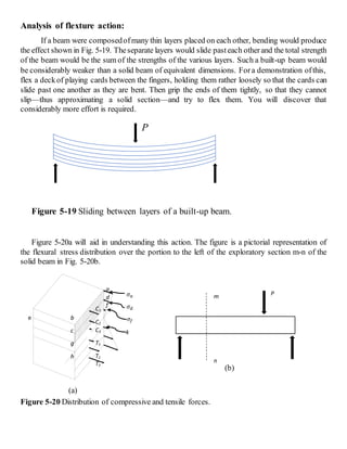
Figure 5-20a will aid in understanding this action. The figure is a pictorial representation of
the flexural stress distribution over the portion to the left of the exploratory section m-n of the
solid beam in Fig. 5-20b.
(b)
Figure 5-20 Distribution of compressive and tensile forces.
P
e b
c
g
h
C1
C2
C3
T3
T2
T3
𝜎 𝑎
𝜎 𝑑
𝜎𝑓
k
a
d
f
Pm
n
(a)

2. If we add the horizontal forces acting over the entire depth of the section, the compressive
forces will exactly balance the tensile forces, as is required by the equilibrium condition ∑Fx= 0
.However, if we take a summation of horizontal forces over a partial depth of the section, say,
from the top element a-b to thoseat c-d, the total compressive force C₁ over the area abcd (equal
to the area abcd multiplied by the average of the stresses σa and σd) can be balanced only by a
shear resistance developed at the horizontal layer dce. Such shear resistance is available in a solid
beam but not in a built-up beam of unconnected layers.
If we extend the summation ofhorizontal forces downto layer fg, the resultant compressive
forceis increased by C2 , which is the average of the stresses σd and σf multiplied bythe area cdfg.
Thus a larger shear resistance must be developed over the horizontal layer at fg than at dce. Of
course, the total compressive force C1 plus C2 acting over the area abgfmay also be computed as
the average of the stresses σa and σf multiplied by the area abgf. However, the first method
indicates the decreasing magnitude of the increase in the total compressive force as we descend
by equal intervals from the top; that is, although the total compressive force increases as we
descend by equal intervals from the top, it does so by smaller increments.
This analysis shows that the maximum unbalanced horizontal force exists at the neutral
axis. This unbalanced force decreases gradually to zero as the effects of layers the neutral axis
are included. This is so because the horizontal effect of the compressive forces is increasingly
offset by the neutralizing effect of the tensile forces, until finally a complete balance is attained
and ∑Fx = 0 over the entire section.
This analysis also indicates that layers equidistant from the neutral axis, such as fg and hk,
are subject to the same net horizontal unbalance, becausein adding the horizontal forces from the
top to these layers the equal compressive forces C3 and T3 cancel out. We conclude that equal
shear resistances are developed at layers fg and hk. However, this requires that the areas from the
neutral axis to the equidistant layers be symmetrical with respect to the neutral axis. The
conclusion would not hold, for example, if the beam section were a triangle with its base
horizontal.
DERIVATION OF FORMULA FOR HORIZONTAL SHEARING STRESS:
Consider two adjacent sections, (1) and (2), in a beam separated by the distance dx, as
shown in Fig. 5-21, and let the shaded part between them be isolated as a free body. Figure 5-22
is a pictorial representation of this part, the beam from which it is taken being shown in dashed
outline.
Assume the bending moment at section (2) to be larger than that at section (l), thus causing
larger flexural stresses onsection (2) than on section (1). Therefore, the resultant horizontal thrust

3. H2 caused by the compressive forces on section (2) will be greater than the resultant horizontal
thrust H1 on section (l). This difference between H2 and H1 can be balanced only by the resisting
shear force dF acting on the bottom face of the free body, since no external force acts on the top
or side faces of the free body.
y
b
c
𝑦1
dxSection (1) Section (2)
c
𝐻1
𝑦1
𝐻2
Resisting shear
dF = 𝜏𝑏𝑑𝑥
⇁
Figure 5-21
Section (1)
Section (1)
𝜎1 𝑑𝐴
𝜎2 𝑑𝐴
y
Figure 5-22

4. Since H2 — H1 is the summation of the differences in thrusts σ2 dA and σ1 dA on the ends of all
elements contained in the part shown in Fig. 5-22, a horizontal summation of forces gives
[∑FH = 0] dF = H2 – H1
=∫ 𝜎2
dA
𝑐
𝑦1
– ∫ 𝜎1
dA
𝑐
𝑦1
Replacing the flexural stress σ by its equivalent My/l, we obtain
dF =
𝑀2
𝐼
∫ 𝑦dA
𝑐
𝑦1
–
𝑀1
𝐼
∫ 𝑦dA
𝑐
𝑦1
=
𝑀2− 𝑀1
𝐼
∫ 𝑦dA
𝑐
𝑦1
From Fig. 5-21 we note that dF = 𝜏b dx, where 𝜏 is the average shearing stress over the
differential area of width b and length dx; also that M2 – M1 represents the differential change in
bending moment dM in the distance dx; hence the preceding relation is rewritten as
𝜏 =
𝑑𝑀
𝐼𝑏 𝑑𝑥
∫ 𝑦dA
𝑐
𝑦1
From Art. 4-4 we recall that dM/dx= V, the vertical shear; so we obtain for the horizontal
shearing stress
𝝉 =
𝑽
𝑰𝒃
∫ 𝒚𝐝𝐀
𝒄
𝒚 𝟏
=
𝑽
𝑰𝒃
A′𝒚̅ =
𝑽
𝑰𝒃
𝑸 (5-4)
We have replaced the integral ∫ 𝑦dA
𝑐
𝑦1
, which means the sum of the moments of the
differential areas dA about the neutral axis, by its equivalent A′𝑦̅, where A′ is the partial area of
the section above the layer at which the shearing stress is being computed and 𝑦̅ is the moment
arm of this area with respect to the neutral axis; A′ is the shaded area in the end view of Fig. 5-
21. A variation ofthe product A′𝑦̅ is the symbol Q, which frequently is used to represent the static
moment of area.
Shear Flow
If the shearing stress 𝜏 is multiplied by the width b, we obtain a quantity q, known as shear
flow, which represents the longitudinal forceunit length transmitted across thesection at the level
y1. It is analogous to the shear flow discussed previously in the torsionof thin-walled tubes, Using
Eq. (5-4), we find that its value is given by
Q = 𝝉b =
𝑽
𝑰𝒃
𝑸 (5-4a)
Relation Between Horizontal and Vertical Shearing Stresses:

5. Most students are surprised to find the term vertical shear (V) appearing in the formula for
horizontal shearing stress (𝜏h). However, as we shall show presently, a horizontal shearing stress
is always accompanied by an equal vertical shearing stress. It is this vertical shearing stress 𝜏v,
shown in Fig. 5-23, that forms the resisting vertical shear Vr =∫ 𝜏𝑑𝐴 which balances the vertical
shear V. Since it is not feasible to determine 𝜏v directly, we have resorted to deriving the
numerically equal value of 𝜏h .
Figure 5-23 Horizontal and vertical shearing stresses.
To prove the equivalence of 𝜏h and 𝜏v, consider their effect on a free-body diagram of a
typical element in fig. 5-23. A pictorial view of this element is shown in Fig. 5-24a; a front
view, in Fig. 5-24b. For of this element, the shearing stress 𝜏h on the bottom face requires an
equal balancing shearing stress On the top face. The forces causing these shearing streses (fig.
5-23c) form
x
z
y
𝜏ℎ
𝜏 𝑣
𝑉𝑟 = ∫ 𝜏𝑑𝐴

6. a counterclockwise couple, which requires a clockwise couple to ensure balance. The
forces of this clockwise couple induce the shearing stresses 𝜏v on the vertical faces of the
element as shown.
By taking moments about an axis through A (Fig. 5-24c), we obtain
[ ∑ MA = 0] (𝜏v dx dz)dy - (𝜏v dy dz)dx = 0
from which the constant product dx dy dz is canceled to yield
𝝉h = 𝝉v (5-5)
We conclude therefore that a shearing stress acting on one face of an element is always
accompanied by a numerically equal shearing stress acting on a perpendicular face.
Application to Rectangular Section
The distribution of shearing stresses in a rectangular section can be obtained by applying
Eq. (5-4) to Fig. 5-25. For a layer at a distance y from the neutral axis, we have
𝜏 =
𝑉
𝐼𝑏
A′𝑦̅ =
𝑉
𝐼𝑏
[ b(
ℎ
2
- y)][ y +
1
2
(
ℎ
2
- y)]
↿ ↿
↼ ↼↿ ↿
↼ ↼
dy
dx
dz
𝜏ℎ
𝜏ℎ
𝜏 𝑣
𝜏 𝑣
𝜏 𝑣 𝜏 𝑣
𝜏 𝑣dy
dz
𝜏ℎ
𝜏ℎ 𝜏ℎ 𝑑𝑥𝑑𝑧
dy
dx
A
(b)
Stresses
(c)
Forces
(a)
Figure 5-24 Shearing stresses on a typical element

7. which reduces to
𝜏 =
𝑉
2𝐼
(
ℎ2
4
– y2)
This shows that the shearing stress is distributed parabolically across the depth of the section.
The maximum shearing stress occurs at the neutral axis and is found by substituting the
dimensions of the rectangle in Eq. (5-4), as follows:
𝜏 =
𝑉
𝐼𝑏
A′𝑦̅ =
𝑉
(
𝑏ℎ3
12
) 𝑏
(
𝑏ℎ
2
)(
ℎ
4
)
Which reduces to
Max. 𝝉 =
𝟑
𝟐
𝑽
𝒃𝒉
=
𝟑
𝟐
𝑽
𝑨
(5-6)
This indicates that the maximum shearing stress in a rectangular section is 50% greater than the
average shear stress.
Assumptions and Limitations of Formula
We have assumed, without saying so implicitly, that the shearing stress is uniform across
the width ofthe cross section. Although this assumption does nothold rigorously, it is sufficiently
accurate for sections in which the flexure forces are evenly distributed over a horizontal layer.
NA
h/2
y
h
b
Figure 5-25 Shearing stress is distributed parabolically across a rectangular section

8. Figure 5-26
This condition is present in a rectangular section and in the wide-flange section shown in
Fig. 5-26a, where the flexure forces on the vertical strips, both shaded and unshaded, are evenly
distributed across any horizontal layer. But this condition does not exist in the triangular section
in Fig. 5-26b, where the shearing stress is maximum at the left edge of the neutral axis,
diminishing to zero at the right edge. Even here, however, Eq. (5-4) can be used to compute the
average value of shearing stress across any layer. Another exception is a circular cross section
(Fig. 5-26c) It can be shown that the stress at the edge of any layer must tangent to the surface.
as in the right half of the figure; but the direction of shearing at interior is unknown, although
they are assumed to through a common center C as shown. The vertical components of these
sharing are usually assumed to uniform across any layer, as in the left half of the figure, and are
computed by means of Eq. (5-4). With this assumption, the maximum shearing stress across the
neutral axis is
4
3
(
𝑃
𝜋𝑟2
). A more elaborate study shows that shearing stress actually varies at the
neutral axis from 1.23
𝑃
𝜋𝑟2
at the edges to 1.38
𝑃
𝜋𝑟2
at the center.
5-8 DESIGN FOR FLEXURE AND SHEAR
In this article we consider the determination of load capacity or the size of beam section
that will satisfy allowable stresses in both flexure and shear. No principles are required beyond
those already developed.
In heavily loaded short beams the design is usually governed by the shearing stress (which
varies with V); but in longer beams the flexure stress generally governs because the bending
moment varies with both load and length of beam. Shearing is more important in timber beams
than in steel beams because of the low shearing strength of wood.