MTCS TOPIC

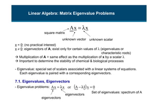
1. x
x
A λ
=
Linear Algebra: Matrix Eigenvalue Problems
x = 0: (no practical interest)
x ≠ 0: eigenvectors of A; exist only for certain values of λ (eigenvalues or
characteristic roots)
 Multiplication of A = same effect as the multiplication of x by a scalar λ
 Important to determine the stability of chemical & biological processes
- Eigenvalue: special set of scalars associated with a linear systems of equations.
Each eigenvalue is paired with a corresponding eigenvectors.
7.1. Eigenvalues, Eigenvectors
- Eigenvalue problems:
square matrix
eigenvectors
unknown scalar
( ) 0
x
I
A
or
x
x
A =
λ
−
λ
=
unknown vector
eigenvectors
Set of eigenvalues: spectrum of A

2. How to Find Eigenvalues and Eigenvectors
Ex. 1.)






−
−
=
2
2
2
5
A
2
2
1
1
2
1
x
x
2
x
2
x
x
2
x
5
λ
=
−
λ
=
+
−
( ) 0
x
I
A =
λ
−
In homogeneous linear system, nontrivial solutions exist when det (A-λI)=0.
0
6
7
2
2
2
5
)
I
A
det(
)
(
D 2
=
+
λ
+
λ
=
λ
−
−
λ
−
−
=
λ
−
=
λ
Characteristic equation of A:
Characteristic determinant
Characteristic polynomial
Eigenvalues: λ1=-1 and λ2= -6
Eigenvectors: for λ1=-1, for λ2=-6,






=
2
1
x1 





−
=
1
2
x2
obtained from Gauss elimination

3. General Case
Theorem 1:
Eigenvalues of a square matrix A  roots of the characteristic equation of A.
nxn matrix has at least one eigenvalue, and at most n numerically different eigenvalues.
Theorem 2:
If x is an eigenvector of a matrix A, corresponding to an eigenvalue λ,
so is kx with any k≠0.
Ex. 2) multiple eigenvalue
- Algebraic multiplicity of λ: order Mλ of an eigenvalue λ
Geometric multiplicity of λ: number of mλ of linear independent eigenvectors
corresponding to λ. (=dimension of eigenspace of λ)
In general, mλ ≤ Mλ
Defect of λ: Δλ=Mλ-mλ
n
n
nn
2
2
n
1
1
n
1
n
n
1
2
12
1
11
x
x
a
x
a
x
a
x
x
a
x
a
x
a
λ
=
+
+
+
λ
=
+
+
+



( ) ( ) 0
I
A
det
)
(
D
,
0
x
I
A =
λ
−
=
λ
=
λ
−

4. 7.2. Some Applications of Eigenvalue Problems
Ex. 1) Stretching of an elastic membrane.
Find the principal directions: direction of position vector x of P
= (same or opposite) direction of the position vector y of Q














=






=
=
+
2
1
2
1
2
2
2
1
x
x
5
3
3
5
y
y
y
,
1
x
x








−
=
=








=
=

=
=
1
1
for
x
,
2
1
1
for
x
,
8
x
x
A
y
2
2
2
1
1
1
λ
λ
λ
λ
λ
Eigenvalue represents speed of response
Eigenvector ~ direction

5. Ex. 4) Vibrating system of two masses on two springs
Solution vector:
solve eigenvalues and eigenvectors
2
1
'
'
2
2
1
'
'
1
y
2
y
2
y
y
2
y
5
y
−
=
+
−
=
wt
e
x
y =
)
t
6
sin
b
t
6
cos
a
(
x
)
t
sin
b
t
cos
a
(
x
y
)
w
(
x
x
A
2
2
2
1
1
1
2
+
+
+
=

=
=
 λ
λ

7. 7.3. Symmetric, Skew-Symmetric, and Orthogonal Matrices
- Three classes of real square matrices
(1) Symmetric:
(2) Skew-symmetric:
(3) Orthogonal:
Theorem 1:
(a) The eigenvalues of a symmetric matrix are real.
(b) The eigenvalues of a skew-symmetric matrix are pure imaginary or zero.










−
−
−
−
=
−
=
0
20
12
20
0
9
12
9
0
,
a
a
,
A
A jk
kj
T










−
−
−
=
=
4
2
5
2
0
1
5
1
3
,
a
a
,
A
A jk
kj
T
















−
−
=
−
3
2
3
2
3
1
3
1
3
2
3
2
3
2
3
1
3
2
,
A
A
1
T
( )
( ) symmetric
skew
A
A
2
1
S
symmetric
A
A
2
1
R
,
S
R
A
T
T
−
−
=
+
=
+
=
Zero-diagonal terms
)
real
,
A
A
(
k
k
A
k
k
A
:
Conjugate
k
k
A =
=

=
= λ
λ
λ
Transpose, and then multiply k: k
k
k
k
k
k
k
k
k
k
k
A
k
T
T
T
T
T
T
T
λ
λ
λ
λ
λ =

=

=

8. Ex. 3)
Orthogonal Transformations and Matrices
- Orthogonal transformation in the 2D plane and 3D space: rotation
Theorem 2: (Invariance of inner product)
An orthogonal transformation preserves the value of the inner product of vectors.
the length or norm of a vector in Rn given by
Theorem 3: (Orthonormality of column and row vectors)
A real square matrix is orthogonal iff its column (or row) vectors, a1,… , an form an
orthonormal system
i
25
,
0
0
20
12
20
0
9
12
9
0
±
=
λ










−
−
−
)
matrix
orthogonal
:
A
(
x
A
y =
8
,
2
5
3
3
5
=
λ






















θ
θ
θ
−
θ
=








=
2
1
2
1
x
x
cos
sin
sin
cos
y
y
y
)
Ex
)
vectors
column
:
b
,
a
(
b
a
b
a
T
=
⋅
a
a
a
a
a
T
=
⋅
=




=
≠
=
=
⋅
k
j
if
1
k
j
if
0
a
a
a
a k
T
j
k
j
b
a
b
a
b
)
A
A
(
a
b
A
A
a
)
b
A
(
)
a
A
(
v
u
v
u
)
orthogonal
:
A
(
b
A
v
,
a
A
u
T
1
T
T
T
T
T
⋅
=
=
=
=
=
=
⋅
=
=
−
( )
n
1
T
n
T
1
T
1
a
a
a
a
,
A
A
I
A
A 













=
=
−

9. Theorem 4: The determinant of an orthogonal matrix has the value of +1 or –1.
Theorem 5: Eigenvalues of an orthogonal matrix A are real or complex conjugates in
pairs and have absolute value 1.
7.4. Complex Matrices: Hermitian, Skew-Hermitian, Unitary
- Conjugate matrix:
- Three classes of complex square matrices:
(1) Hermitian:
(2) Skew-Hermitian:
(3) Unitary:
kj
T
jk a
A
,
a
A =
=








+
−
−
=









−
−
−
+
=
i
2
6
i
5
7
i
4
3
A
i
2
6
7
i
5
i
4
3
A
T






+
−
=
=
7
i
3
1
i
3
1
4
,
a
a
,
A
A jk
kj
T






−
+
−
+
−
=
−
=
i
i
2
i
2
i
3
,
a
a
,
A
A jk
kj
T










=
−
i
2
1
3
2
1
3
2
1
i
2
1
,
A
A
1
T
Diagonal-terms: real
Diagonal-terms:
pure imag. or 0
2
T
T
1
)
A
(det
A
det
A
det
)
A
A
det(
)
A
A
det(
I
det
1 =
=
=
=
=
−
jj
jj a
a =
jj
jj a
a −
=

10. - Generalization of section 7.3
Hermitian matrix: real  symmetric
Skew-Hermitian matrix: real  skew-symmetric
Unitary matrix: real  orthogonal
Eigenvalues
Theorem 1:
(a) Eigenvalues of Hermitian (symmetric) matrix  real
(b) Skew-Hermitian (skew-symmetric) matrix  pure imag. or zero
(c) Unitary (orthogonal) matrix  absolute value 1
Forms
: a form in the components x1,… , xn of x, A coefficient matrix
A
A
A
T
T
=
=
A
A
A
T
T
−
=
=
1
T
T
A
A
A
−
=
=
x
A
x
T
[ ] 2
2
22
1
2
21
2
1
12
1
1
11
2
1
22
21
12
11
2
1
T
x
x
a
x
x
a
x
x
a
x
x
a
x
x
a
a
a
a
x
x
x
A
x +
+
+
=












=
Re λ
Im λ
Skew-Hermitian
Hermitian
Unitary

11. Proof of Theorem 1:
(a) Eigenvalues of Hermitian (symmetric) matrix  real
(b) Eigenvalues of Skew-Hermitian (skew-symmetric) matrix  pure imag. or zero
(c) Eigenvalues of Unitary (orthogonal) matrix  absolute value 1
( ) ( )
x
A
x
x
A
x
x
A
x
x
A
x
x
A
x
)
A
A
,
A
A
use
(
!
real
?
real
x
x
x
A
x
x
x
x
x
x
A
x
x
x
A
T
T
T
T
T
T
T
T
T
T
T
T
T
T
=
=
=
=
=
=
=
=
=
=

=
λ
λ
λ
λ
( )
x
A
x
x
A
x
T
T
−
=
( ) ( )
( ) ( ) ( ) ( ) x
x
x
x
x
x
x
x
x
A
x
A
x
x
A
:
transpose
conjugate
x
x
A
T
T
2
T
T
T
T
T
=
=
=
=
=

=
λ
λ
λ
λ
λ
λ
λ

12. n
n
nn
1
n
1
n
n
2
n
2
1
2
21
n
1
n
1
1
1
11
n
1
j
n
1
k
k
j
jk
T
x
x
a
x
x
a
x
x
a
x
x
a
x
x
a
x
x
a
x
x
a
x
A
x
+
+
+
+
+
+
+
+
+
=
= 
= =









- For general n,
- For real A, x,
Quadratic form
- Hermitian A: Hermitian form, Skew-Hermitian A: Skew-Hermitian form
Theorem 1: For every choice of the vector x, the value of a Hermitian form is real,
and the value of a skew-Hermitian form is pure imaginary or 0.
2
n
nn
2
n
2
n
1
n
1
n
n
2
n
2
2
2
22
1
2
21
n
1
n
1
2
1
12
2
1
11
n
1
j
n
1
k
k
j
jk
T
x
a
x
x
a
x
x
a
x
x
a
x
a
x
x
a
x
x
a
x
x
a
x
a
x
x
a
x
A
x
+
+
+
+
+
+
+
+
+
+
=
= 
= =










13. Properties of Unitary Matrices. Complex Vector Space Cn.
- Complex vector space: Cn
Inner product:
length or norm:
Theorem 2: A unitary transformation, y=Ax (A: unitary matrix) preserves the value of
the inner product and norm.
- Unitary system: complex analog of an orthonormal system of real vectors
Theorem 3: A square matrix is unitary iff its column vectors form a unitary system.
Theorem 4: The determinant of a unitary matrix has absolute value 1.
b
a
b
a
T
=
⋅
2
n
2
1
T
a
a
a
a
a
a
a +
+
=
=
⋅
= 




=
≠
=
=
⋅
k
j
if
1
k
j
if
0
a
a
a
a k
T
j
k
j
b
a
b
a
b
A
A
a
)
b
A
(
)
a
A
(
v
u
v
u
T
T
T
T
T
⋅
=
=
=
=
=
⋅
2
T
T
1
A
det
A
det
A
det
A
det
A
det
A
det
A
det
)
A
A
det(
)
A
A
det(
I
det
1
=
=
=
=
=
=
=
−

14. 7.5. Similarity of Matrices, Basis of Eigenvectors, Diagonalization
-Eigenvectors of n x n matrix A forming a basis for Rn or Cn ~ used for diagonalizing A
Similarity of Matrices
- n x n matirx is similar to an n x n matrix A if for nonsingular n x n P
Similarity transformation:
Theorem 1: has the same eigenvalues as A if is similar to A.
is an eigenvector of corresponding to the same eigenvalue,
if x is an eigenvector of A.
Properties of Eigenvectors
Theorem 2: λ1, λ2, …, λn: distinct eigenvalues of an n x n matrix.
Corresponding eigenvectors x1, x2, …, xn  a linearly independent set.
( ) ( )
x
P
x
P
Â
x
P
P
A
P
x
I
A
P
x
A
P
x
P
x
A
P
x
x
A
1
1
1
1
1
1
1
1
−
−
−
−
−
−
−
−
=
=
=
=
=

=
λ
λ
λ
P
A
P
Â
1
−
=
Â
A
from
Â
 Â
x
P
y
1
−
= Â

15. Theorem 3: n x n matrix A has n distinct eigenvalues  A has a basis of eigenvector
for Cn (or Rn).
Ex. 1)
Theorem 4: A Hermitian, skew-Hermitian, or unitary matrix has a basis of
eigenvectors for Cn that is a unitary system.
A symmetric matrix has an orthonomal basis of eigenvectors for Rn.
Ex. 3) From Ex. 1, orthonormal basis of eigenvectors
- Basis of eigenvectors of a matrix A: useful in transformation and diagonalization
Complicated calculation of A on x  sum of simple evaluation on the eigenvectors of A.






−












=
1
1
,
1
1
rs
eigenvecto
of
basis
a
5
3
3
5
A








−








2
/
1
2
/
1
,
2
/
1
2
/
1
( )
n
n
n
1
1
1
n
n
2
2
1
1
n
1
n
n
2
2
1
1
x
c
x
c
x
c
x
c
x
c
A
y
)
basis
:
x
...,
,
x
(
x
c
x
c
x
c
x
,
x
A
y
λ
λ +
+
=
+
+
+
=

+
+
+
=
=



( ) 2
1
2
T
1
2
1
2
T
1
2
2
T
1
1
2
T
1
2
2
2
T
1
2
T
1
T
1
2
T
1
1
2
1
T
1
2
T
T
1
1
T
1
T
T
1
2
2
T
1
2
1
2
2
2
)
2
(
1
1
1
)
1
(
,
x
x
0
x
x
x
x
x
x
x
x
x
A
x
:
left
the
on
x
Multiply
)
2
(
x
x
x
x
x
A
x
x
A
x
:
right
the
on
x
multiply
then
,
Transpose
)
1
(
0
x
x
x
x
show
;
x
x
A
,
x
x
A
λ
λ
λ
λ
λ
λ
λ
λ
λ
λ
λ
λ
λ
≠
−
=

=
=
=
=
=
→
=
=
=
⋅
=
=

16. Diagonalization
Theorem 5: If an n x n matrix A has a basis of eigenvectors, then
is diagonal, with the eigenvalues of A on the main diagonal.
(X: matrix with eigenvectors as column vectors)
 n x n matrix A is diagonalizable iff A has n linearly independent eigenvectors.
 Sufficient condition for diagonalization: If an n x n matrix A has n distinct
eigenvalues, it is diagonalizable.
Ex. 4)
Ex. 5) Diagonalization
X
A
X
D
1
−
=
...)
,
3
,
2
m
(
X
A
X
D
m
1
m
=
=
−






=






−
=






−












=
−
1
0
0
6
X
A
X
;
1
1
1
4
X
;
1
1
,
1
4
rs
eigenvecto
;
2
1
4
5
A
1
[ ] [ ] [ ]
X
A
X
X
A
A
X
X
A
X
X
A
X
D
D
X
A
X
D
X
x
x
x
A
x
A
x
x
A
X
A
2
1
1
1
1
2
1
n
n
1
1
n
1
n
1
−
−
−
−
−
=
=
=
=

=
=
=
= λ
λ 


x1,…,xn: basis of eigenvectors of A for Cn (or Rn) corresponding to λ1, …, λn

17. Transformation of Forms to Principal Axes
Quadratic form:
If A is real symmetric, A has an orthogonal basis of n eigenvectors
 X is orthogonal.
Theorem 6: The substitution x=Xy, transforms a quadratic form
to the principal axes form
where λ1,…, λn eigenvalues of the symmetric Matrix A, and X is
orthogonal matrix with corresponding eigenvectors as column vectors.
Ex. 6) Conic sections.
x
A
x
Q
T
=
1
T
X
X
−
= T
1
X
D
X
X
D
X
A =
=
−
( )
y
X
x
,
x
X
x
X
y
y
y
y
y
D
y
x
X
D
X
x
Q
1
T
2
n
n
2
n
1
2
1
1
T
T
T
=
=
=
+
+
+
=
=
=
−
λ
λ
λ 

= =
=
=
n
1
j
n
1
k
k
j
jk
T
x
x
a
x
A
x
Q
2
n
n
2
n
1
2
1
1
T
y
y
y
y
D
y
Q λ
λ
λ +
+
+
=
= 

18. Example) Solution of linear 1st-order Eqn.:
Ex.)
)
0
(
y
X
e
X
)
t
(
z
X
)
t
(
y
)
0
(
z
e
z
z
D
z
)
0
(
z
)
0
(
z
e
0
0
e
)
t
(
z
)
t
(
z
z
z
0
0
z
z
z
D
z
z
X
A
z
X
y
X
z
z
X
y
:
Define
y
A
dt
y
d
y
1
t
D
t
D
2
1
t
t
2
1
2
1
2
1
2
1
1
2
1
−
−
=
=

=

=














=





















=






=
→
=
=
→
=
=
=







λ
λ
λ
λ
2
2
2
1
1
y
2
y
y
y
5
.
0
y
−
=
+
−
=


)
0
(
y
8321
.
0
0
5547
.
0
1
e
0
0
e
8321
.
0
0
5547
.
0
1
)
t
(
y
2
for
8321
.
0
5547
.
0
y
,
5
.
0
for
0
1
y
1
t
2
t
5
.
0
2
2
1
1
−
−
−







 −















 −
=
−
=





−
=
−
=






=
 λ
λ