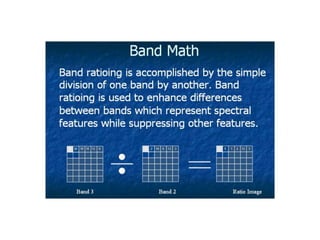
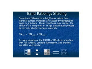
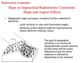
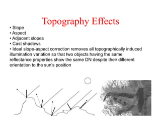
Image Enhancement
• To improve the visual interpretability of an
image by increasing the apparent distinction
between the features of the scene
• This objective is to create new image from
the original image in order to increase the
amount of information that can be visually
interpreted from the data
• Enhancement operations are normally
applied to image data after the appropriate
restoration procedures have been performed
Image Enhancement
• Point operations:
– modify the brightness value of each pixel
independently
• Local operations:
– modify the value of each pixel based on
neighboring brightness values
Image Enhancement
• Follows noise removal
1. Contrast manipulation
– Thresholding
– Stretching
– Slicing
Image Enhancement
2. Spatial feature manipulation
– Filtering
– Edge enhancement
– Fourier analysis
3. Multi-image manipulation
Gray-Level Thresholding
• To segment the image into two classes
• One having pixels values below an analyst-
defined gray level and one for pixels above
this value
• Many objects or image regions are
characterized by constant reflectivity or
light absorption of their surface; a brightness
constant or threshold can be determined to
segment objects and background.
Slicing
• Gray levels (DN) distributed along the x axis
of an image histogram are divided into a
series of analyst-specified intervals (slices)
• All DNs falling within a given interval are
displayed at a single DN in the output image
• The process of converting the continuous grey
tone of an image into a series of density
intervals, or slices, each corresponding to a
specific digital range
Slicing
Contrast Stretching
• To expand the narrow range of brightness values of an input
image over a wider range of gray values
• Certain features may reflect more energy than others. This
results in good contrast within the image and features that are
easy to distinguish
• The contrast level between the features in an image is low
when features reflect nearly the same level of energy
• When image data are acquired, the detected energy does not
necessarily fill the entire grey level range that the sensor is
capable of. This can result in a large concentration of values in
a small region of grey levels producing an image with very
little contrast among the features.
Contrast Stretching
Contrast Stretching
• Stretch the contrast to enhance features interested
– Linear stretch
• A radiometric enhancement technique that improves the contrast of an
image for visual interpretation purposes
• A linear stretch occurs, when the grey level values of an image are
uniformly stretched across a larger display range
• Usually, the original minimum and maximum grey level values are set
to the lowest and highest grey level values in the display range,
respectively
• For example, if the maximum grey level value in the original image is
208 and the minimum grey level value was 68, the ‘stretched’ values
would be set at 255 and 0 respectively
– Non-linear
• A radiometric enhancement technique that stretches the range of
image brightness in a non-proportional manner
• A nonlinear stretch expands one portion of the grey scale while
compressing the other portion
Contrast Stretching
• Linear stretch:
Where
DN’= Digital no. assigned to pixel in output image
DN= Original DN of pixel in input image
MIN= Minimum value of input image (0)
MAX=Maximum value of input image (255)

DN' ( DNMIN
MAXMIN )255
Linear stretch
Example of linear stretching
Linear Stretch
Non-linear
Contrast Stretching
• Histogram-equalized stretch: An image
processing technique that displays the most
frequently occurring image values.
• The brightest regions of the image will be
assigned a larger range of DN values so that
radiometric detail is enhanced
Histogram-equalized stretch
Spatial Filtering
• Filters are commonly used for such
things as edge enhancement, noise
removal, and the smoothing of high
frequency data
• The principle of the various filters is
to modify the numerical value of
each pixel as a function of the
neighbouring pixels’ values.
• For example, if the value of each
pixel is replaced by the average of its
value and those of its eight
neighbours the image is smoothed,
that is to say, the finer details
disappear and the image appears
fuzzier.
• For example, the filtered value of the
pixel located at E5 is
(9*1/9) + (5*1/9) + (5*1/9) + (9*1/9)
+ (5*1/9) + (5*1/9) + (5*1/9) +
(5*1/9) + (5*1/9) = 5.89, rounded up
to 6.
Spatial Feature Manipulation
• Spatial filters pass (emphasize) or suppress (de-emphasize) image data of various
spatial frequencies
• Spatial frequency refers to the number of changes in brightness value, per unit
distance, for any area within a scene
• Spatial frequency corresponds to image elements (both important details and
noise) of certain size
• High spatial frequency  rough areas
– High frequency corresponds to image elements of smallest size
– An area with high spatial frequency will have rapid change in digital values
with distance (i.e. dense urban areas and street networks)
• Low spatial frequency  smooth areas
– Low frequency corresponds to image elements of (relatively) large size.
– An object with a low spatial frequency only changes slightly over many
pixels and will have gradual transitions in digital values (i.e. a lake or a
smooth water surface).
Spatial Filtering
• The neighbourhood
• The image profile
• Numerical filters
– low-pass filters
– high-pass filters
The Neighbourhood
• A resampling technique that calculates the brightness value
of a pixel in a corrected image from the brightness value
of the pixel nearest the location of the pixel in the input image
B: Kernel or neighborhood
Around a target pixel (A)
Spatial Filtering
16 12 20
13 9 15
2 7 12
12
Input Output
(16*1/9) + (12*1/9) + (20*1/9) + (13*1/9) + (9*1/9) + (15*1/9) + (2*1/9) + (7*1/9) + (12*1/9) = 12
The Image Profile
Image profiles show the data values across an image
line (X), column (Y), or spectral bands (Z).
High and Low Frequency Changes
Numerical Filters-Low Pass Filters
– Extract low frequency
information (long wavelength)
– Suppress high frequency
information (short wavelength)
– low pass filter contains the same
weights in each kernel element,
replacing the center pixel value
with an average of the
surrounding values
– Low pass filters are useful in
smoothing an image, and reduce
"salt and pepper" (speckle) noise
from SAR images.
1 1 1
1 1 1
1 1 1
Low-pass Filters
Low-pass Filters
Details are “smoothed” and DNs
are averaged after a low pass
filter is applied to an image.
Detail is lost, but noisy images
and “speckle” in SAR images are
smoothed out.
Numerical Filters-High Pass Filters
– Are used for removing , for
example, stripe noise of low
frequency (low energy, long
short wavelengths)
– Filters that pass high
frequencies (short wavelength)
– high pass filter uses a 3 x 3
kernel with a value of 8 for the
center pixel and values of -1
for the exterior pixels
– It can be used to enhance
edges between different
regions as well as to sharpen an
image
-1 -1 -1
-1 8 -1
-1 -1 -1
High-pass Filter
High-pass Filter
Streets and highways, and some
streams and ridges, are greatly
emphasized. The trademark of a
high pass filter image is that
linear features commonly are
defined as bright lines with a
dark border.
Convolution
• A moving window is established, containing
an array of coefficients or weighting factors
called operators or kernels
– (odd number: 3 x 3, …)
• The kernel (window around the target
pixel) is moved throughout the original
image and a new, convoluted image results
from its application
Edge Enhancement
• Edge-enhanced images attempt to preserve
local contrast and low-frequency brightness
information, for example related to linear
features such as roads, canals, geological
faults, etc.
Edge Enhancement
• Edge enhancement is typically implemented in three
steps:
– High-frequency component image is produced using the
appropriate kernel size. Rough images suggest small filter size
(e.g. 3 × 3 pixels) whereas large sizes (e.g. 9 × 9) are used with
smooth images
– All or a fraction of the gray level in each pixel is added back to
high-frequency component image
– The composite image is contrast-stretched
Directional First Differencing
• Directional First Differencing is another
enhancement technique aimed to enhance
edges in image data
• Compares each pixel in an image to one of
its adjacent neighbors and displays the
difference as gray levels of an output image
Directional First Differencing
A H
V D
Horizontal first difference= DNA-DNH
Vertical first difference= DNA-DNV
Diagonal first difference= DNA-DND
Directional First Differencing
Multi-Image Manipulation
• Spectral rationing
• Ratio images are enhancements resulting
from the division of DNs in one spectral band
by the corresponding values in another band.
Ratio Images
• Used for discriminating subtle spectral variations
that are masked by the brightness variations
• Depends on the particular reflectance
characteristics of the features involved and the
application at hand
Ratio Images
• Ratio images can also be used to generate
false color composites by combining three
monochromatic ratio data sets.
• Advantage: combining data from more than
two bands and presenting the data in color
Steps in Impractical Radiometric Correction:
Slope and Aspect Effects
• Topographic slope and aspect introduce further radiometric
distortion.
– Local variation in view and illumination angles
– Identical surface objects might be represented by
totally different intensity values
The goal of topographic
correction is to remove all
topographically caused variance,
so that areas with the same
reflectance have the same
radiance or reflectance
(depending on the analysis)
Radiometric Correction
Topography Effects
• Slope
• Aspect
• Adjacent slopes
• Cast shadows
• Ideal slope-aspect correction removes all topographically induced
illumination variation so that two objects having the same
reflectance properties show the same DN despite their different
orientation to the sun’s position
Topographic Normalization
• Ratioing (Lillesand and Kiefer)
– not taking into account physical behavior of scene elements
• Lambertian surface
– not valid assumption
– Normalisation according to the cosine of effective
llumination angle
• Non-lambertian behaviour
– Additional parameters added
– Estimated by regression between distorted band and DEM
Ratio Images
• Hybrid color ratio composite:
– two ratio images in two primary colors, and using
the third primary color to display a regular band
of data.
Linear Data Transformations
• The individual bands are often observed to
be highly correlated or redundant.
• Two mathematical transformation techniques
are often used to minimize this spectral
redundancy:
– principal component analysis (PCA)
– canonical analysis (CA)
Principal Components Analysis
• Compute a set of new, transformed variables
(components), with each component largely
independent of the others (uncorrelated).
• The components represent a set of mutually
orthogonal and independent axes in a n-dimensional
space.
– The first new axis contains the highest percentage of the
total variance or scatter in the data set.
– Each succeeding (lower-order) axis containing less variance
PCA and CA
Rotation of axes in 2-dimensional space for a hypothetical two-band
data set by principal components analysis (left) and canonical analysis
(right). PCA uses DN information from the total scene, whereas CA uses
the spectral characteristics of categories defined within the data to
increase their separability.
PC Images
Principal & Canonical
Components
• Problem:
– Multispectral remote sensing datasets comprise a
set of variables (the spectral bands), which are
usually correlated to some extent
– That is, variations in the DN in one band may be
mirrored by similar variations in another band
(when the DN of a pixel in Band 1 is high, it is also
high in Band 3, for example).
Principal & Canonical
Components
• Solution:
– Principal Component Analysis (PCA) is used to produce
uncorrelated output bands and to determine/reduce the data
dimensionality
– Principal and canonical component transformations, applied
either as an enhancement operation prior to the visual
interpretation or as preprocessing procedure prior to
automated classification of data
– PCA “Bands” produce more colorful color composite images
than spectral color composite images using normal
wavelength bands because the variance in the data has been
maximized.
– By selecting which PCA Bands to exclude in further
processing, you can reduce the amount of data you are
handling, eliminate noise, and reduce computational
requirements.
Principal & Canonical
Components
• To compress all information contained in a n-
band dataset into less than n components
(new bands)
• Scatter diagrams
• Principal components and new axes
Principal & Canonical
Components
• To compress all information contained in a n-
band dataset into less than n components
(new bands)
• Scatter diagrams
• Principal components and new axes
Principal & Canonical
Components
• To compress all information contained in a n-
band dataset into less than n components
(new bands)
• Scatter diagrams
• Principal components and new axes
Accuracy Assessment: Reference
Data
• Issue 2: Determining size of reference
plots
– Take into account spatial frequencies of
image
– E.G. For the two examples below, consider
photo reference plots that cover an area 3
pixels on a side
Example 1: Low
spatial frequency
Homogeneous image
Example 2: High
spatial frequency
Heterogenous image
Accuracy Assessment: Reference
Data
• Issue 2: Determining size of reference plots
– HOWEVER, also need to take into account
accuracy of position of image and reference data
– E.G. For the same two examples, consider the
situation where accuracy of position of the image
is +/- one pixel
Example 1: Low
spatial frequency
Example 2: High
spatial frequency

12-Image enhancement and filtering.ppt

  • 1.
    Image Enhancement • Toimprove the visual interpretability of an image by increasing the apparent distinction between the features of the scene • This objective is to create new image from the original image in order to increase the amount of information that can be visually interpreted from the data • Enhancement operations are normally applied to image data after the appropriate restoration procedures have been performed
  • 2.
    Image Enhancement • Pointoperations: – modify the brightness value of each pixel independently • Local operations: – modify the value of each pixel based on neighboring brightness values
  • 3.
    Image Enhancement • Followsnoise removal 1. Contrast manipulation – Thresholding – Stretching – Slicing
  • 4.
    Image Enhancement 2. Spatialfeature manipulation – Filtering – Edge enhancement – Fourier analysis 3. Multi-image manipulation
  • 5.
    Gray-Level Thresholding • Tosegment the image into two classes • One having pixels values below an analyst- defined gray level and one for pixels above this value • Many objects or image regions are characterized by constant reflectivity or light absorption of their surface; a brightness constant or threshold can be determined to segment objects and background.
  • 6.
    Slicing • Gray levels(DN) distributed along the x axis of an image histogram are divided into a series of analyst-specified intervals (slices) • All DNs falling within a given interval are displayed at a single DN in the output image • The process of converting the continuous grey tone of an image into a series of density intervals, or slices, each corresponding to a specific digital range
  • 7.
  • 8.
    Contrast Stretching • Toexpand the narrow range of brightness values of an input image over a wider range of gray values • Certain features may reflect more energy than others. This results in good contrast within the image and features that are easy to distinguish • The contrast level between the features in an image is low when features reflect nearly the same level of energy • When image data are acquired, the detected energy does not necessarily fill the entire grey level range that the sensor is capable of. This can result in a large concentration of values in a small region of grey levels producing an image with very little contrast among the features.
  • 9.
  • 10.
    Contrast Stretching • Stretchthe contrast to enhance features interested – Linear stretch • A radiometric enhancement technique that improves the contrast of an image for visual interpretation purposes • A linear stretch occurs, when the grey level values of an image are uniformly stretched across a larger display range • Usually, the original minimum and maximum grey level values are set to the lowest and highest grey level values in the display range, respectively • For example, if the maximum grey level value in the original image is 208 and the minimum grey level value was 68, the ‘stretched’ values would be set at 255 and 0 respectively – Non-linear • A radiometric enhancement technique that stretches the range of image brightness in a non-proportional manner • A nonlinear stretch expands one portion of the grey scale while compressing the other portion
  • 11.
    Contrast Stretching • Linearstretch: Where DN’= Digital no. assigned to pixel in output image DN= Original DN of pixel in input image MIN= Minimum value of input image (0) MAX=Maximum value of input image (255)  DN' ( DNMIN MAXMIN )255
  • 12.
  • 13.
  • 14.
  • 15.
  • 17.
    Contrast Stretching • Histogram-equalizedstretch: An image processing technique that displays the most frequently occurring image values. • The brightest regions of the image will be assigned a larger range of DN values so that radiometric detail is enhanced
  • 18.
  • 19.
    Spatial Filtering • Filtersare commonly used for such things as edge enhancement, noise removal, and the smoothing of high frequency data • The principle of the various filters is to modify the numerical value of each pixel as a function of the neighbouring pixels’ values. • For example, if the value of each pixel is replaced by the average of its value and those of its eight neighbours the image is smoothed, that is to say, the finer details disappear and the image appears fuzzier. • For example, the filtered value of the pixel located at E5 is (9*1/9) + (5*1/9) + (5*1/9) + (9*1/9) + (5*1/9) + (5*1/9) + (5*1/9) + (5*1/9) + (5*1/9) = 5.89, rounded up to 6.
  • 20.
    Spatial Feature Manipulation •Spatial filters pass (emphasize) or suppress (de-emphasize) image data of various spatial frequencies • Spatial frequency refers to the number of changes in brightness value, per unit distance, for any area within a scene • Spatial frequency corresponds to image elements (both important details and noise) of certain size • High spatial frequency  rough areas – High frequency corresponds to image elements of smallest size – An area with high spatial frequency will have rapid change in digital values with distance (i.e. dense urban areas and street networks) • Low spatial frequency  smooth areas – Low frequency corresponds to image elements of (relatively) large size. – An object with a low spatial frequency only changes slightly over many pixels and will have gradual transitions in digital values (i.e. a lake or a smooth water surface).
  • 21.
    Spatial Filtering • Theneighbourhood • The image profile • Numerical filters – low-pass filters – high-pass filters
  • 22.
    The Neighbourhood • Aresampling technique that calculates the brightness value of a pixel in a corrected image from the brightness value of the pixel nearest the location of the pixel in the input image B: Kernel or neighborhood Around a target pixel (A)
  • 23.
    Spatial Filtering 16 1220 13 9 15 2 7 12 12 Input Output (16*1/9) + (12*1/9) + (20*1/9) + (13*1/9) + (9*1/9) + (15*1/9) + (2*1/9) + (7*1/9) + (12*1/9) = 12
  • 24.
    The Image Profile Imageprofiles show the data values across an image line (X), column (Y), or spectral bands (Z).
  • 25.
    High and LowFrequency Changes
  • 26.
    High and LowFrequency Changes
  • 27.
    Numerical Filters-Low PassFilters – Extract low frequency information (long wavelength) – Suppress high frequency information (short wavelength) – low pass filter contains the same weights in each kernel element, replacing the center pixel value with an average of the surrounding values – Low pass filters are useful in smoothing an image, and reduce "salt and pepper" (speckle) noise from SAR images. 1 1 1 1 1 1 1 1 1
  • 28.
  • 29.
    Low-pass Filters Details are“smoothed” and DNs are averaged after a low pass filter is applied to an image. Detail is lost, but noisy images and “speckle” in SAR images are smoothed out.
  • 30.
    Numerical Filters-High PassFilters – Are used for removing , for example, stripe noise of low frequency (low energy, long short wavelengths) – Filters that pass high frequencies (short wavelength) – high pass filter uses a 3 x 3 kernel with a value of 8 for the center pixel and values of -1 for the exterior pixels – It can be used to enhance edges between different regions as well as to sharpen an image -1 -1 -1 -1 8 -1 -1 -1 -1
  • 31.
  • 32.
    High-pass Filter Streets andhighways, and some streams and ridges, are greatly emphasized. The trademark of a high pass filter image is that linear features commonly are defined as bright lines with a dark border.
  • 33.
    Convolution • A movingwindow is established, containing an array of coefficients or weighting factors called operators or kernels – (odd number: 3 x 3, …) • The kernel (window around the target pixel) is moved throughout the original image and a new, convoluted image results from its application
  • 35.
    Edge Enhancement • Edge-enhancedimages attempt to preserve local contrast and low-frequency brightness information, for example related to linear features such as roads, canals, geological faults, etc.
  • 36.
    Edge Enhancement • Edgeenhancement is typically implemented in three steps: – High-frequency component image is produced using the appropriate kernel size. Rough images suggest small filter size (e.g. 3 × 3 pixels) whereas large sizes (e.g. 9 × 9) are used with smooth images – All or a fraction of the gray level in each pixel is added back to high-frequency component image – The composite image is contrast-stretched
  • 37.
    Directional First Differencing •Directional First Differencing is another enhancement technique aimed to enhance edges in image data • Compares each pixel in an image to one of its adjacent neighbors and displays the difference as gray levels of an output image
  • 38.
    Directional First Differencing AH V D Horizontal first difference= DNA-DNH Vertical first difference= DNA-DNV Diagonal first difference= DNA-DND
  • 39.
  • 40.
    Multi-Image Manipulation • Spectralrationing • Ratio images are enhancements resulting from the division of DNs in one spectral band by the corresponding values in another band.
  • 43.
    Ratio Images • Usedfor discriminating subtle spectral variations that are masked by the brightness variations • Depends on the particular reflectance characteristics of the features involved and the application at hand
  • 44.
    Ratio Images • Ratioimages can also be used to generate false color composites by combining three monochromatic ratio data sets. • Advantage: combining data from more than two bands and presenting the data in color
  • 45.
    Steps in ImpracticalRadiometric Correction: Slope and Aspect Effects • Topographic slope and aspect introduce further radiometric distortion. – Local variation in view and illumination angles – Identical surface objects might be represented by totally different intensity values The goal of topographic correction is to remove all topographically caused variance, so that areas with the same reflectance have the same radiance or reflectance (depending on the analysis) Radiometric Correction
  • 46.
    Topography Effects • Slope •Aspect • Adjacent slopes • Cast shadows • Ideal slope-aspect correction removes all topographically induced illumination variation so that two objects having the same reflectance properties show the same DN despite their different orientation to the sun’s position
  • 47.
    Topographic Normalization • Ratioing(Lillesand and Kiefer) – not taking into account physical behavior of scene elements • Lambertian surface – not valid assumption – Normalisation according to the cosine of effective llumination angle • Non-lambertian behaviour – Additional parameters added – Estimated by regression between distorted band and DEM
  • 48.
    Ratio Images • Hybridcolor ratio composite: – two ratio images in two primary colors, and using the third primary color to display a regular band of data.
  • 49.
    Linear Data Transformations •The individual bands are often observed to be highly correlated or redundant. • Two mathematical transformation techniques are often used to minimize this spectral redundancy: – principal component analysis (PCA) – canonical analysis (CA)
  • 50.
    Principal Components Analysis •Compute a set of new, transformed variables (components), with each component largely independent of the others (uncorrelated). • The components represent a set of mutually orthogonal and independent axes in a n-dimensional space. – The first new axis contains the highest percentage of the total variance or scatter in the data set. – Each succeeding (lower-order) axis containing less variance
  • 51.
    PCA and CA Rotationof axes in 2-dimensional space for a hypothetical two-band data set by principal components analysis (left) and canonical analysis (right). PCA uses DN information from the total scene, whereas CA uses the spectral characteristics of categories defined within the data to increase their separability.
  • 52.
  • 53.
    Principal & Canonical Components •Problem: – Multispectral remote sensing datasets comprise a set of variables (the spectral bands), which are usually correlated to some extent – That is, variations in the DN in one band may be mirrored by similar variations in another band (when the DN of a pixel in Band 1 is high, it is also high in Band 3, for example).
  • 55.
    Principal & Canonical Components •Solution: – Principal Component Analysis (PCA) is used to produce uncorrelated output bands and to determine/reduce the data dimensionality – Principal and canonical component transformations, applied either as an enhancement operation prior to the visual interpretation or as preprocessing procedure prior to automated classification of data – PCA “Bands” produce more colorful color composite images than spectral color composite images using normal wavelength bands because the variance in the data has been maximized. – By selecting which PCA Bands to exclude in further processing, you can reduce the amount of data you are handling, eliminate noise, and reduce computational requirements.
  • 56.
    Principal & Canonical Components •To compress all information contained in a n- band dataset into less than n components (new bands) • Scatter diagrams • Principal components and new axes
  • 57.
    Principal & Canonical Components •To compress all information contained in a n- band dataset into less than n components (new bands) • Scatter diagrams • Principal components and new axes
  • 58.
    Principal & Canonical Components •To compress all information contained in a n- band dataset into less than n components (new bands) • Scatter diagrams • Principal components and new axes
  • 59.
    Accuracy Assessment: Reference Data •Issue 2: Determining size of reference plots – Take into account spatial frequencies of image – E.G. For the two examples below, consider photo reference plots that cover an area 3 pixels on a side Example 1: Low spatial frequency Homogeneous image Example 2: High spatial frequency Heterogenous image
  • 60.
    Accuracy Assessment: Reference Data •Issue 2: Determining size of reference plots – HOWEVER, also need to take into account accuracy of position of image and reference data – E.G. For the same two examples, consider the situation where accuracy of position of the image is +/- one pixel Example 1: Low spatial frequency Example 2: High spatial frequency