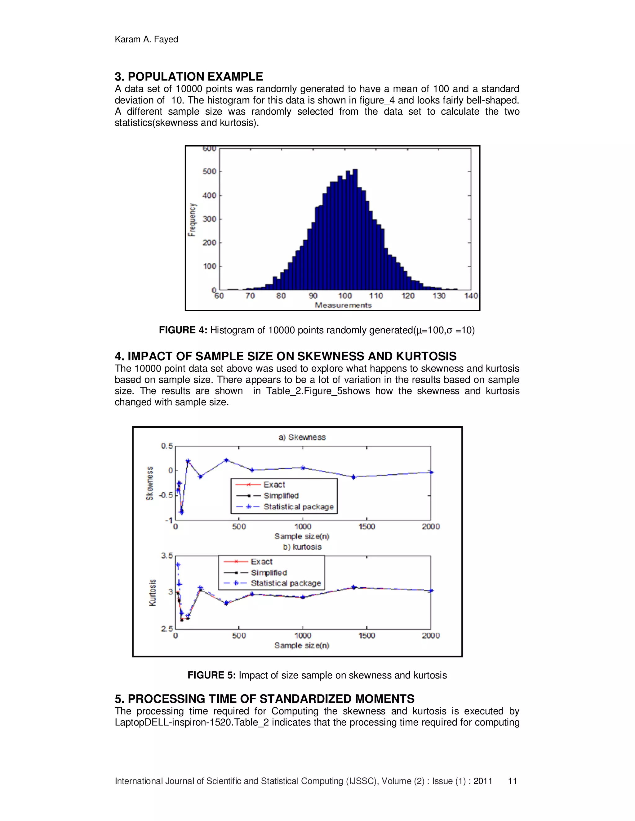
The document presents an optimal algorithm for computing standardized moments, particularly skewness and kurtosis, using MATLAB, boasting a remarkable 99.95% reduction in computational energy compared to existing methods. It discusses the significance of moments in statistical analysis, error analysis, and performance metrics while comparing conventional and simplified techniques based on sample sizes. The findings suggest that the simplified method is preferable, especially for small sample sizes, due to lower error rates and reduced computational demands.

1. Karam A. Fayed
International Journal of Scientific and Statistical Computing (IJSSC), Volume (2) : Issue (1) : 2011 1
Optimum Algorithm for Computing the Standardized Moments
Using MATLAB 7.10(R2010a)
K.A.Fayed karamfayed_1@hotmail.com
Ph.D.From Dept. of applied Mathematics and
Computing, Cranfield University, UK.
Faculty of commerce/Dept. of applied Statistics and Computing,
Port Said University, Port Fouad, Egypt.
Abstract
A fundamental task in many statistical analyses is to characterize the location and variability
of a data set. A further characterization of the data includes skewness and kurtosis. This
paper emphasizes the real time computational problem for generally the r
th
standardized
moments and specially for both skewness and kurtosis. It has therefore been important to
derive an optimum computational technique for the standardized moments. A new algorithm
has been designed for the evaluation of the standardized moments. The evaluation of error
analysis has been discussed. The new algorithm saved computational energy by
approximately 99.95%than that of the previously published algorithms.
Keywords:Statistical Toolbox, Mathematics, MATLAB Programming
1. INTRODUCTION
The formula used for Z –score appears in two virtually identical forms, recognizing the fact
that we may be dealing with sample statistics or population parameters. These formulae are
as follow:
s
xx
z i
i
−
= Sample statistics (1)
σ
µ−
= i
i
x
Z Population statistics (2)
Where:
ix a row score to be standardized
n sample size
∑=
=
n
i
ix
n
x
1
1
Sample mean
µ Population mean
s Sample standard deviation
σ Population standard deviation
z Sample z score
Z Populationz score.
Subtracting the mean centers the distribution and dividing by the standard normalizes the
distribution. The interesting properties of Z score are that they have a zero mean (effect of
centering) and a variance and standard of one (effect of normalizing). We can use Z score to
compare samples coming from different distributions [1].
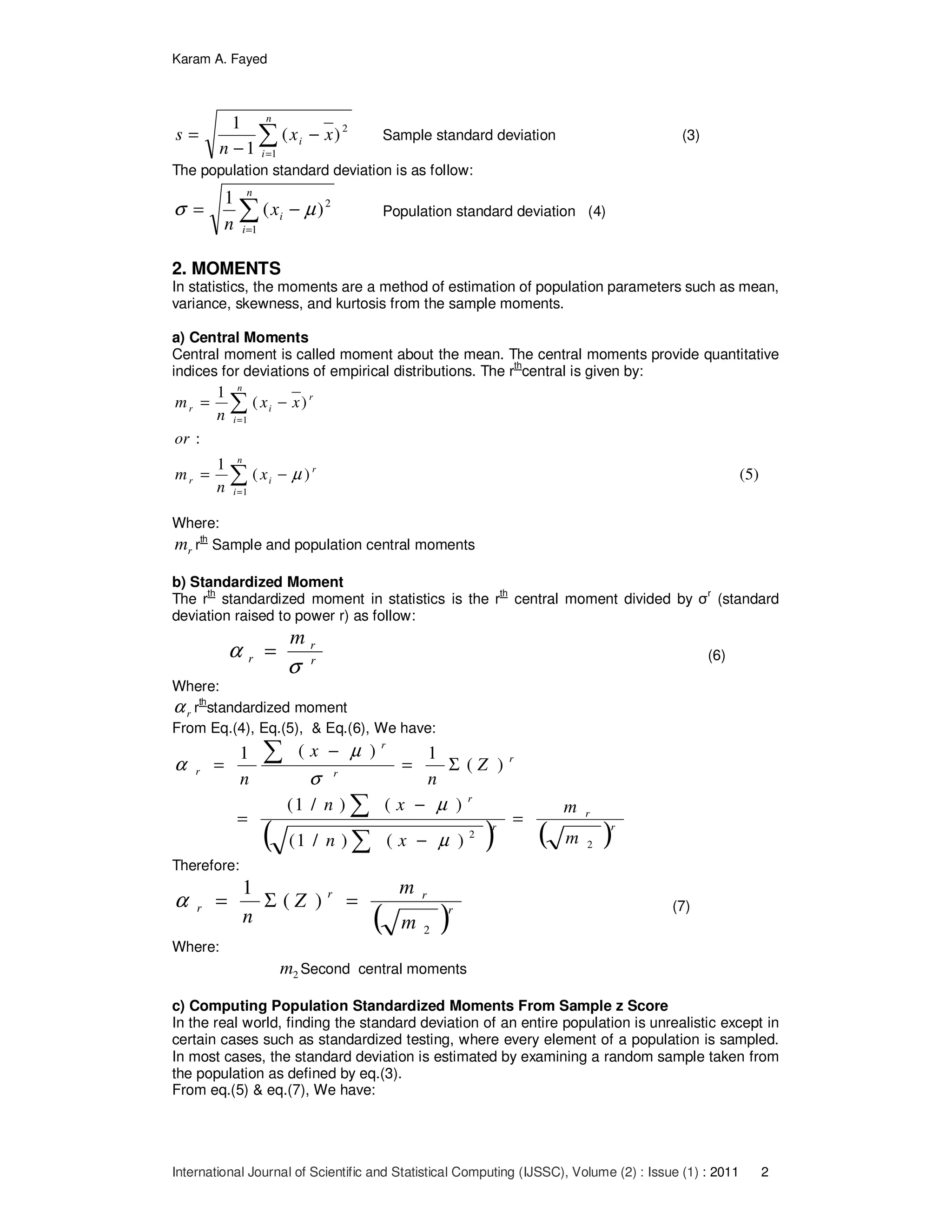
The most common and useful measure of dispersion is the standard deviation. The formula
for sample standard deviation is as follow:

2. Karam A. Fayed
International Journal of Scientific and Statistical Computing (IJSSC), Volume (2) : Issue (1) : 2011 2
∑=
−
−
=
n
i
i xx
n
s
1
2
)(
1
1
Sample standard deviation (3)
The population standard deviation is as follow:
∑=
−=
n
i
ix
n 1
2
)(
1
µσ Population standard deviation (4)
2. MOMENTS
In statistics, the moments are a method of estimation of population parameters such as mean,
variance, skewness, and kurtosis from the sample moments.
a) Central Moments
Central moment is called moment about the mean. The central moments provide quantitative
indices for deviations of empirical distributions. The r
th
central is given by:
(5))(
1
:
)(
1
1
1
∑
∑
=
=
−=
−=
n
i
r
ir
n
i
r
ir
x
n
m
or
xx
n
m
µ
Where:
rm r
th
Sample and population central moments
b) Standardized Moment
The r
th
standardized moment in statistics is the r
th
central moment divided by σ
r
(standard
deviation raised to power r) as follow:
r
r
r
m
σ
α = (6)
Where:
rα r
th
standardized moment
From Eq.(4), Eq.(5), & Eq.(6), We have:
( ) ( )r
r
r
r
r
r
r
r
m
m
xn
xn
Z
n
x
n
2
2
)()/1(
)()/1(
)(
1)(1
=
−
−
=
Σ=
−
=
∑
∑
∑
µ
µ
σ
µ
α
Therefore:
( )r
rr
r
m
m
Z
n
2
)(
1
=Σ=α (7)
Where:
2m Second central moments
c) Computing Population Standardized Moments From Sample z Score
In the real world, finding the standard deviation of an entire population is unrealistic except in
certain cases such as standardized testing, where every element of a population is sampled.
In most cases, the standard deviation is estimated by examining a random sample taken from
the population as defined by eq.(3).
From eq.(5) & eq.(7), We have:

3. Karam A. Fayed
International Journal of Scientific and Statistical Computing (IJSSC), Volume (2) : Issue (1) : 2011 3
( )r
rr
r
m
m
Z
n
2
)(
1
=Σ=α
( )r
r
xxn
xxn
∑
∑
−
−
=
2
)()/1(
)()/1(
( ) 2/22/2/
)1/()()1()/1(
)()/1(
rrr
r
nxxnn
xxn
∑
∑
−−−
−
=
( )
∑
∑
∑






−
=
−





−
=
−
−
=
r
r
rr
r
rr
r
z
n
n
n
Sxx
n
n
n
Snn
xxn
2/
2/
2/22/
1
1
/)(
1
1
)/)1((
)()/1(
Therefore:
∑





−
= r
rl
r z
n
n
n
2
1
1
α (8)
Equation(8) represents the general equation for computing the rth
standardized moments of
sample z-score.
d) Simplified Standardized Moments
From eq.(8), the term
2
1
1
rl
n
n
n






−
can be simplified using binomial theorem, since it
can obtain the binomial series which is valid for any real number as follow:
The term
2
1
1
rl
n
n
n






−
can be rewritten in the following form:
222
1
1
111
1
1
rlrlrl
nnn
n
nn
n
n
−−






−=




 −
=





−
(10)
By replacing and we have:
For large values of ,we get:

4. Karam A. Fayed
International Journal of Scientific and Statistical Computing (IJSSC), Volume (2) : Issue (1) : 2011 4
Substituting Eq.(12) in eq.(8), we get:
Where:
r
th
simplified standardized moments.
e) Mathematical Formulae of Standardized and Simplified Moments
Using Eq.(8) & Eq.(13), we can get the following formulae:
Name r
th
Standardized moments Simplified moments
Mean 1
Variance 2
Skewness 3
Kurtosis 4
f) Ratio Between Population and Sample z-Score
From Eq.(7) & Eq.(8), we can get the exact and simplified ratio of population and sample z-
score as follow:
Since:
We get:
And from Eq.(7) & Eq.(13), we can get:
Eq.(14) and Eq.(15) appear to be very dependent on the sample size. Therefore the ratio
between population and sample z-score(required for computing ther
th
standardized moments)
depends on the sample size as given in Table_1. This table shows the variation. Figure_1
shows that the sample z score gets closer to population Z score. Therefore, computing
standardized moments using simplified technique is recommended for small sample size.

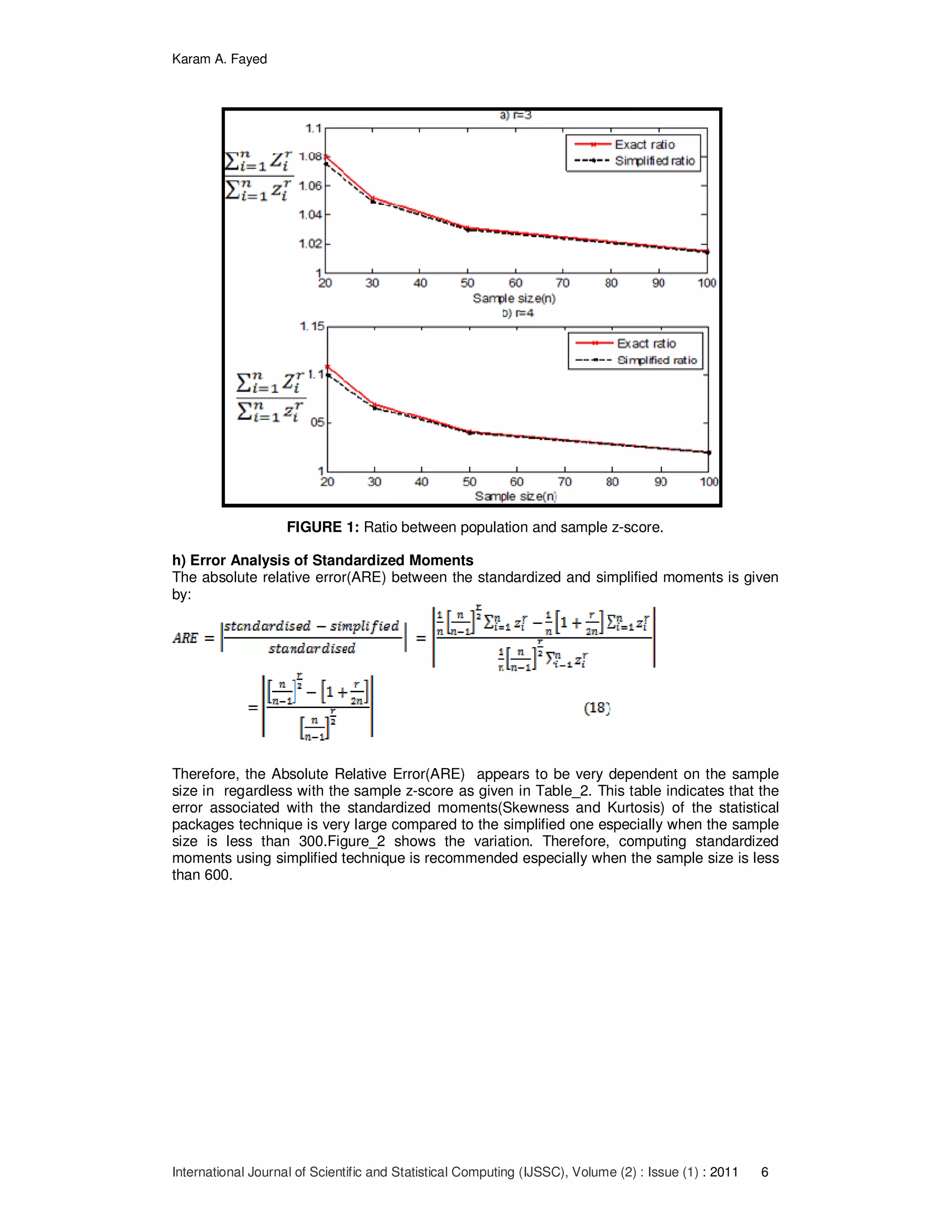
5. Karam A. Fayed
International Journal of Scientific and Statistical Computing (IJSSC), Volume (2) : Issue (1) : 2011 5
g) Formulae of Skewness and Kurtosis Applied in Statistical Packages
The usual estimators of the population skewness and kurtosis used in Minitab, SAS, SPSS,
and Excel are defined as follow [2], [3],[4]:
Where:
is the sample standard deviation.
is the usual estimator of population skewness.
is known as the excess kurtosis(without adding 3).
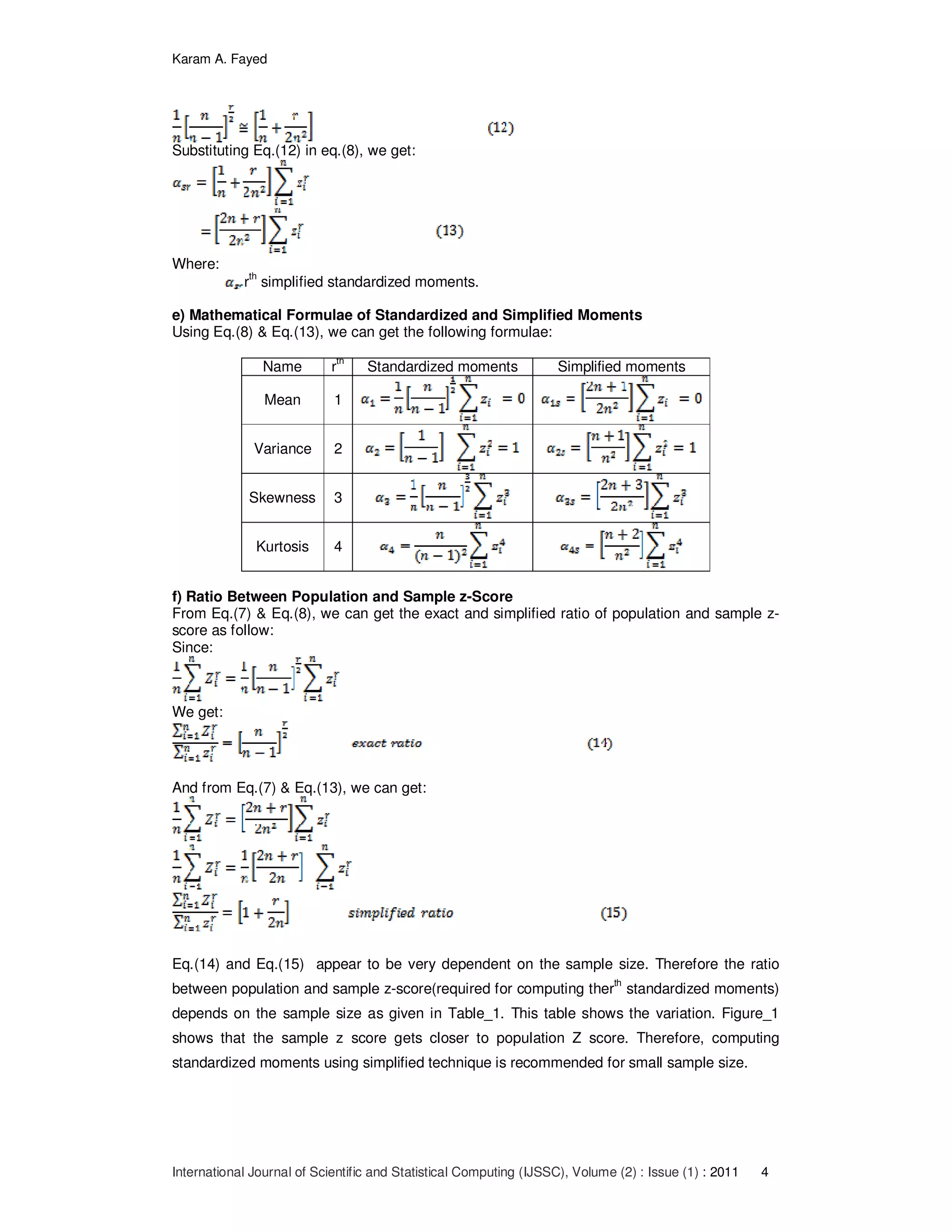
Sample size(n)
Exact ratio Simplified ratio
r=3 r=4 r=3 r=4
20 1.07998 1.10803 1.07500 1.10000
30 1.05217 1.07015 1.05000 1.06667
50 1.03077 1.04123 1.03000 1.04000
100 1.01519 1.02030 1.01500 1.02000
200 1.00755 1.01008 1.00750 1.01000
400 1.00376 1.00502 1.00375 1.00500
600 1.00251 1.00334 1.00250 1.00333
1000 1.00150 1.00200 1.00150 1.00200
1400 1.00107 1.00143 1.00107 1.00143
2000 1.00075 1.00100 1.00075 1.00100
2600 1.00058 1.00077 1.00058 1.00077
3000 1.00050 1.00067 1.00050 1.00066
3600 1.00042 1.00056 1.00042 1.00055
4000 1.00038 1.00050 1.00038 1.00050
4500 1.00033 1.00044 1.00033 1.00044
5000 1.00030 1.00040 1.00030 1.00040
5500 1.00027 1.00036 1.00027 1.00036
6000 1.00025 1.00033 1.00025 1.00033
8000 1.00019 1.00025 1.00019 1.00025
10000 1.00015 1.00020 1.00015 1.00020
TABLE 1: Ratio between population and sample z-score

6. Karam A. Fayed
International Journal of Scientific and Statistical Computing (IJSSC), Volume (2) : Issue (1) : 2011 6
FIGURE 1: Ratio between population and sample z-score.
h) Error Analysis of Standardized Moments
The absolute relative error(ARE) between the standardized and simplified moments is given
by:
Therefore, the Absolute Relative Error(ARE) appears to be very dependent on the sample
size in regardless with the sample z-score as given in Table_2. This table indicates that the
error associated with the standardized moments(Skewness and Kurtosis) of the statistical
packages technique is very large compared to the simplified one especially when the sample
size is less than 300.Figure_2 shows the variation. Therefore, computing standardized
moments using simplified technique is recommended especially when the sample size is less
than 600.

7. Karam A. Fayed
International Journal of Scientific and Statistical Computing (IJSSC), Volume (2) : Issue (1) : 2011 7
Sample
size(n)
Skewness
Absolute Relative Error
(ARE)`
Exact Simplified
Statistical
package
Simplified Statistical
PackagePract. Comp.
20 -0.37911 -0.37736 -0.41057 0.4608 0.4608 8.2977
30 -0.24103 -0.24053 -0.25390 0.2060 0.2060 5.3420
50 -0.81154 -0.81094 -0.83686 0.0744 0.0744 3.1197
100 0.19241 0.19237 0.19535 0.0186 0.0186 1.5293
200 -0.11239 -0.11239 -0.11324 0.0046 0.0046 0.7572
400 0.21474 0.21474 0.21555 0.0011 0.0011 0.3768
600 0.01677 0.01677 0.01682 0.0005 0.0005 0.2508
1000 0.05781 0.05781 0.05790 0.0001 0.0001 0.1502
1400 -0.12846 -0.12846 -0.12860 9.5e-5 9.5e-5 0.10728
2000 -0.02750 -0.02750 -0.02753 4.6e-5 4.6e-5 0.07507
2600 0.03271 0.03271 0.03273 2.7e-5 2.7e-5 0.05773
3000 -0.01793 -0.01793 -0.01795 2.1e-5 2.1e-5 0.05003
3600 -0.02616 -0.02616 -0.02617 1.4e-5 1.4e-5 0.041688
4000 -0.01818 -0.01818 -0.01819 1.1e-5 1.1e-5 0.037517
4500 0.005310 0.005310 0.005312 9.2e-6 9.2e-6 0.033347
5000 -0.04197 -0.04197 -0.04198 7.5e-6 7.5e-6 0.030011
5500 -0.04199 -0.04199 -0.04200 6.2e-6 6.2e-6 0.027282
6000 0.033432 0.033432 0.033440 5.2e-6 5.2e-6 0.025007
8000 -0.00851 -0.00851 -0.00851 2.9e-6 2.9e-6 0.018754
10000 -0.00057 -0.00057 -0.00057 1.8e-6 1.8e-6 0.015002
TABLE 2: a)Skewness (ARE)
Sample
size(n)
CPU time (Second)
Exact Simplified
Statistical
package
20 0.000185 0.000126 0.000146
30 0.000189 0.000133 0.000145
50 0.000200 0.000156 0.000154
100 0.000213 0.000153 0.000163
200 0.000234 0.000181 0.000185
400 0.000301 0.000257 0.000239
600 0.000394 0.000302 0.000357
1000 0.000487 0.000407 0.000457
1400 0.000584 0.000513 0.000518
2000 0.000746 0.000676 0.000690
2600 0.000989 0.000883 0.000909
3000 0.001096 0.001046 0.001002
3600 0.001233 0.001164 0.001162
4000 0.001396 0.001329 0.001375
4500 0.001489 0.001018 0.001355
5000 0.001594 0.001559 0.001574
5500 0.001785 0.001250 0.001683
6000 0.001891 0.001286 0.001916
8000 0.002164 0.001500 0.002286
10000 0.002318 0.001802 0.003122
TABLE 2: a)Skewness(CPU)

8. Karam A. Fayed
International Journal of Scientific and Statistical Computing (IJSSC), Volume (2) : Issue (1) : 2011 8
Sample
size(n)
Kurtosis Absolute Relative Error(ARE)
Exact Simplified Statistical
Package
Simplified Statistical
PackagePract. Comp.
20 3.0034 2.9816 3.377 0.725 0.725 12.439
30 2.897 2.8876 3.1077 0.32593 0.32593 7.2722
50 2.628 2.6249 2.7182 0.1184 0.11840 3.4341
100 2.6438 2.643 2.6878 0.0298 0.0298 1.6648
200 3.0312 3.031 3.0626 0.00747 0.00747 1.0361
400 2.8435 2.8434 2.8566 0.00187 0.00187 0.4634
600 2.967 2.967 2.9768 0.00083 0.00083 0.32998
1000 2.932 2.932 2.938 0.00029 0.00029 0.19384
1400 3.066 3.066 3.071 0.00015 0.00015 0.14793
2000 3.023 3.023 3.027 7.5e-5 7.5e-5 0.1014
2600 2.947 2.947 2.949 4.4e-5 4.4e-5 0.0749
3000 2.963 2.963 2.965 3.3e-5 3.3e-5 0.06553
3600 2.882 2.882 2.884 2.3e-5 2.3e-5 0.05220
4000 2.976 2.976 2.978 1.8e-5 1.8e-5 0.04946
4500 2.952 2.952 2.954 1.4e-5 1.4e-5 0.04341
5000 3.010 3.010 3.011 1.1e-5 1.1e-5 0.04024
5500 2.998 2.998 2.999 9.9e-6 9.9e-6 0.03636
6000 3.073 3.073 3.074 8.3e-6 8.3e-6 0.03454
8000 3.041 3.041 3.042 4.6e-6 4.6e-6 0.02552
10000 2.911 2.911 2.912 2.9e-6 2.9e-6 0.01909
TABLE 2: b) Kurtosis(ARE)
Sample size(n)
CPU time (Second)
Exact Simplified Statistical
Package
20 0.000164 0.000125 0.000187
30 0.000169 0.000127 0.000196
50 0.000170 0.000153 0.000214
100 0.000192 0.000151 0.000216
200 0.000216 0.000176 0.000248
400 0.000290 0.000256 0.000302
600 0.000327 0.000295 0.000363
1000 0.000547 0.000430 0.000457
1400 0.000563 0.000543 0.000554
2000 0.000737 0.000832 0.001109
2600 0.000967 0.000914 0.000962
3000 0.001020 0.000989 0.001173
3600 0.001187 0.001181 0.001231
4000 0.001338 0.000944 0.001073
4500 0.001426 0.001482 0.001643
5000 0.001128 0.001598 0.001619
5500 0.001138 0.001732 0.001868
6000 0.001826 0.001290 0.001893
8000 0.002628 0.001832 0.002436
10000 0.002571 0.001830 0.002922
TABLE 2: b) Kurtosis(CPU)

9. Karam A. Fayed
International Journal of Scientific and Statistical Computing (IJSSC), Volume (2) : Issue (1) : 2011 9
FIGURE 2: Absolute Relative Error of standardized moments
The percentage reduction in Absolute Relative Error between the statistical packages
technique and the simplified one of the standardized moment is given by:
Where:
isthe percentage reduction in Absolute Relative Error between the statistical packages
technique and the simplified one.
Table_3 shows the percentage reduction in Absolute Relative Error between the statistical
packages technique and the simplified one for different sample size. This table indicates that
the simplified technique of the standardized moments gives reduction in ARE by
approximately 96.7% compared to the statistical package technique especially when the
sample size is less than 100.Figure_3 shows the variation.
The squared error(Er) between the standardized and simplified moments is given by:

10. Karam A. Fayed
International Journal of Scientific and Statistical Computing (IJSSC), Volume (2) : Issue (1) : 2011 10
Sample
size(n)
Skewness (r=3) Kurtosis (r=4)
Error
percentage(%)
Error
reduction(%)
Error
percentage(%)
Error
reduction(%)
20 5.553 94.447 5.828 94.172
30 3.856 96.144 4.482 95.518
50 2.385 97.615 3.448 96.552
100 1.216 98.784 1.790 98.210
200 0.608 99.392 0.721 99.279
400 0.292 99.708 0.404 99.596
600 0.199 99.801 0.252 99.748
1000 0.067 99.933 0.150 99.850
1400 0.089 99.911 0.101 99.899
2000 0.061 99.939 0.074 99.926
2600 0.047 99.953 0.059 99.941
3000 0.042 99.958 0.050 99.950
3600 0.034 99.966 0.044 99.956
4000 0.029 99.971 0.036 99.964
4500 0.028 99.972 0.032 99.968
5000 0.025 99.975 0.027 99.973
5500 0.023 99.977 0.027 99.973
6000 0.021 99.979 0.024 99.976
8000 0.015 99.985 0.018 99.982
10000 0.012 99.988 0.015 99.985
Mean 0.73 % 99.27 % 0.879% 99.121%
TABLE 3: Error reduction of standardized moments
FIGURE 3: Error and error reduction of standardized moments

11. Karam A. Fayed
International Journal of Scientific and Statistical Computing (IJSSC), Volume (2) : Issue (1) : 2011 11
3. POPULATION EXAMPLE
A data set of 10000 points was randomly generated to have a mean of 100 and a standard
deviation of 10. The histogram for this data is shown in figure_4 and looks fairly bell-shaped.
A different sample size was randomly selected from the data set to calculate the two
statistics(skewness and kurtosis).
FIGURE 4: Histogram of 10000 points randomly generated(µ=100,σ =10)
4. IMPACT OF SAMPLE SIZE ON SKEWNESS AND KURTOSIS
The 10000 point data set above was used to explore what happens to skewness and kurtosis
based on sample size. There appears to be a lot of variation in the results based on sample
size. The results are shown in Table_2.Figure_5shows how the skewness and kurtosis
changed with sample size.
FIGURE 5: Impact of size sample on skewness and kurtosis
5. PROCESSING TIME OF STANDARDIZED MOMENTS
The processing time required for Computing the skewness and kurtosis is executed by
LaptopDELL-inspiron-1520.Table_2 indicates that the processing time required for computing

12. Karam A. Fayed
International Journal of Scientific and Statistical Computing (IJSSC), Volume (2) : Issue (1) : 2011 12
the skewnessusing the simplified technique is minimum than other especially when the
sample size increases. Figure_6 shows the variation.
FIGURE 6:a) Execution time required for computing skewness
FIGURE 6: b) Execution time required for computing kurtosis
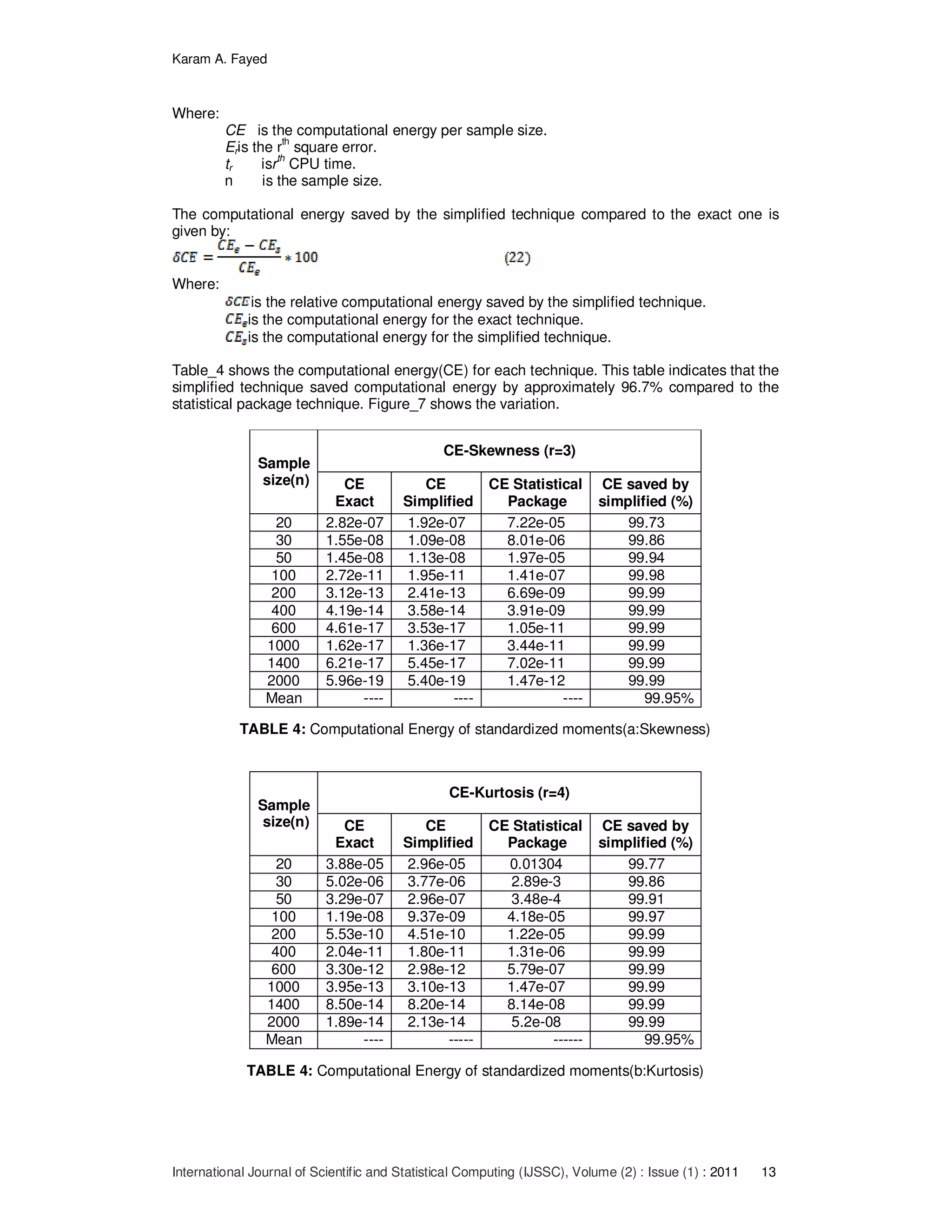
6. COMPUTATIONAL ENERGY OF STANDARDIZED MOMENTS
Computing the computational energy for standardized moments (skewness and kurtosis)
requires the determination of the sample size(n), the square error(Er), and the central
processing time(CPU time). Therefore, consider the sample size(n) represents the resistance,
the square error is measured in [volts]
2
, and the CPU time in second. Then, the computational
energy per sample size is given by:

13. Karam A. Fayed
International Journal of Scientific and Statistical Computing (IJSSC), Volume (2) : Issue (1) : 2011 13
Where:
CE is the computational energy per sample size.
Eris the r
th
square error.
tr isr
th
CPU time.
n is the sample size.
The computational energy saved by the simplified technique compared to the exact one is
given by:
Where:
is the relative computational energy saved by the simplified technique.
is the computational energy for the exact technique.
is the computational energy for the simplified technique.
Table_4 shows the computational energy(CE) for each technique. This table indicates that the
simplified technique saved computational energy by approximately 96.7% compared to the
statistical package technique. Figure_7 shows the variation.
Sample
size(n)
CE-Skewness (r=3)
CE
Exact
CE
Simplified
CE Statistical
Package
CE saved by
simplified (%)
20 2.82e-07 1.92e-07 7.22e-05 99.73
30 1.55e-08 1.09e-08 8.01e-06 99.86
50 1.45e-08 1.13e-08 1.97e-05 99.94
100 2.72e-11 1.95e-11 1.41e-07 99.98
200 3.12e-13 2.41e-13 6.69e-09 99.99
400 4.19e-14 3.58e-14 3.91e-09 99.99
600 4.61e-17 3.53e-17 1.05e-11 99.99
1000 1.62e-17 1.36e-17 3.44e-11 99.99
1400 6.21e-17 5.45e-17 7.02e-11 99.99
2000 5.96e-19 5.40e-19 1.47e-12 99.99
Mean ---- ---- ---- 99.95%
TABLE 4: Computational Energy of standardized moments(a:Skewness)
Sample
size(n)
CE-Kurtosis (r=4)
CE
Exact
CE
Simplified
CE Statistical
Package
CE saved by
simplified (%)
20 3.88e-05 2.96e-05 0.01304 99.77
30 5.02e-06 3.77e-06 2.89e-3 99.86
50 3.29e-07 2.96e-07 3.48e-4 99.91
100 1.19e-08 9.37e-09 4.18e-05 99.97
200 5.53e-10 4.51e-10 1.22e-05 99.99
400 2.04e-11 1.80e-11 1.31e-06 99.99
600 3.30e-12 2.98e-12 5.79e-07 99.99
1000 3.95e-13 3.10e-13 1.47e-07 99.99
1400 8.50e-14 8.20e-14 8.14e-08 99.99
2000 1.89e-14 2.13e-14 5.2e-08 99.99
Mean ---- ----- ------ 99.95%
TABLE 4: Computational Energy of standardized moments(b:Kurtosis)

14. Karam A. Fayed
International Journal of Scientific and Statistical Computing (IJSSC), Volume (2) : Issue (1) : 2011 14
FIGURE 7: Computational Energy for standardized moments
7. MATLAB PROGRAMMING
A complete program can be obtained by writing to the author[4]. There is a part of MATLAB
program shown here:
% Grenrate random data set of size (n) points with mean (mu) and a standard
% deviation (segma)and returns: (1) skewness and kurtosis,(2) cpu time,(3) ARE &
% SquareError,(4) Computational Energy(CE),(5) computational energy saved
% by the simplified technique compared to the exact one
options.Interpreter='tex';
prompt = {'Enter Sample size:','Enter mean(mu) :','Enter std.dev.(sigma) :'};
dlg_title = 'Generate random data set';
num_lines = 1;
def = {'','',''};
options.Resize='on';
options.WindowStyle='normal';
answer = inputdlg(prompt,dlg_title,num_lines,def,options);
ifisempty(answer)
error('No inputs were found!')
end
n=str2num(answer{1})
mu= str2num(answer{2})
sigma = str2num(answer{3})
if n< 3 || isempty(n)
error('n must be integer &>=2')

15. Karam A. Fayed
International Journal of Scientific and Statistical Computing (IJSSC), Volume (2) : Issue (1) : 2011 15
end
// Part of the program is omitted //
tic
S_SP=(n/((n-1)*(n-2)))*sum(((s-mean(s))./std(s)).^r);
t_SP= toc;
tic
S_E=(1/n)*(n/(n-1))^(r/2)*sum((zscore(s)).^r);
t_E = toc;
tic
S_S=(1/n+r/(2*n^2))*sum((zscore(s)).^r);
t_S = toc;
A_E=abs(((S_E-S_S)/S_E)*100);
A_S=abs((((n/(n-1))^(r/2)-(1+r/(2*n)))/(n/(n-1))^(r/2))*100) ;
A_SP=abs(((S_E-S_SP)/S_E)*100);
SK=dataset({ S_E,'Exact'},{ S_S,'Simplified'},{ S_SP,'Stat_Package'} )
ARE=dataset({ A_E,'Practical'},{ A_S,'Computed'}, {A_SP,'Stat_Package'} )
// Part of the program is omitted //
8. CONCLUSIONS
Computer algorithms for fast implementation of standardized moments are an important
continuing area of research.A new algorithm has been designed for the evaluation of the
standardized moments. As a result the new technique offered four advantages over the
current technique:
(1) It drastically reduces the CPU time for calculating the standardized moments
especially when the sample size increases.
(2) It drastically reduces the absolute relative error(ARE) for calculating the
standardized moments(Skewness and Kurtosis) by 99.27% compared to the
current one.
(3) It gives minimum square error compared to the current algorithm.
(4) It has lowest computational energy.
The aforementioned features are combined in a mathematical formula to describe the system
performance. This formula is called the computational energy. A quantitative study has been
carried out to compute the computational energy for each technique. The results show that
the simplified technique saved computational energy by 96.7% compared to the current one.
8. REFERENCES
[1] Neil Salkind, “Encyclopedia of measurement and statistics”, 2007.
[2] D.N.Joanes&C.A.Gill,”Comparing measures of sample skewness and kurtosis”, Journal
of the royal statistical society (series D), Vol.47, No.1,page 183-189, March,1998.
[3] Microsoft Corporation, “Microsoft Office professional plus, Microsoft Excel”, Version
14.0.5128.5000, 2010.
[4] The Mathworks, Inc., MATLAB, the Language of Technical Computing, Version
7.10.0.499 (R2010a), February 5, 2010.
[5] Email: karamfayed_1@hotmail.com