Downloaded 28 times


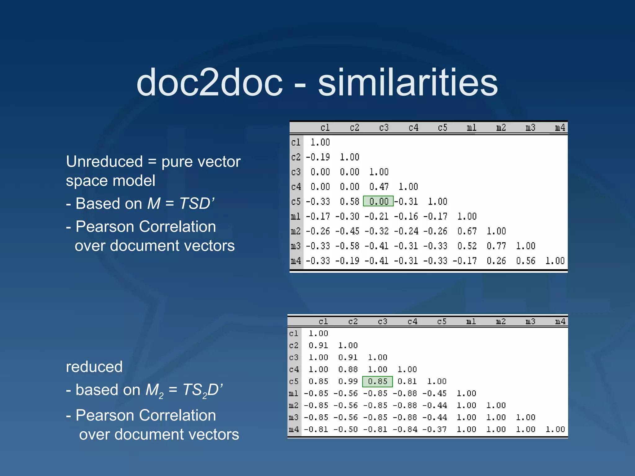
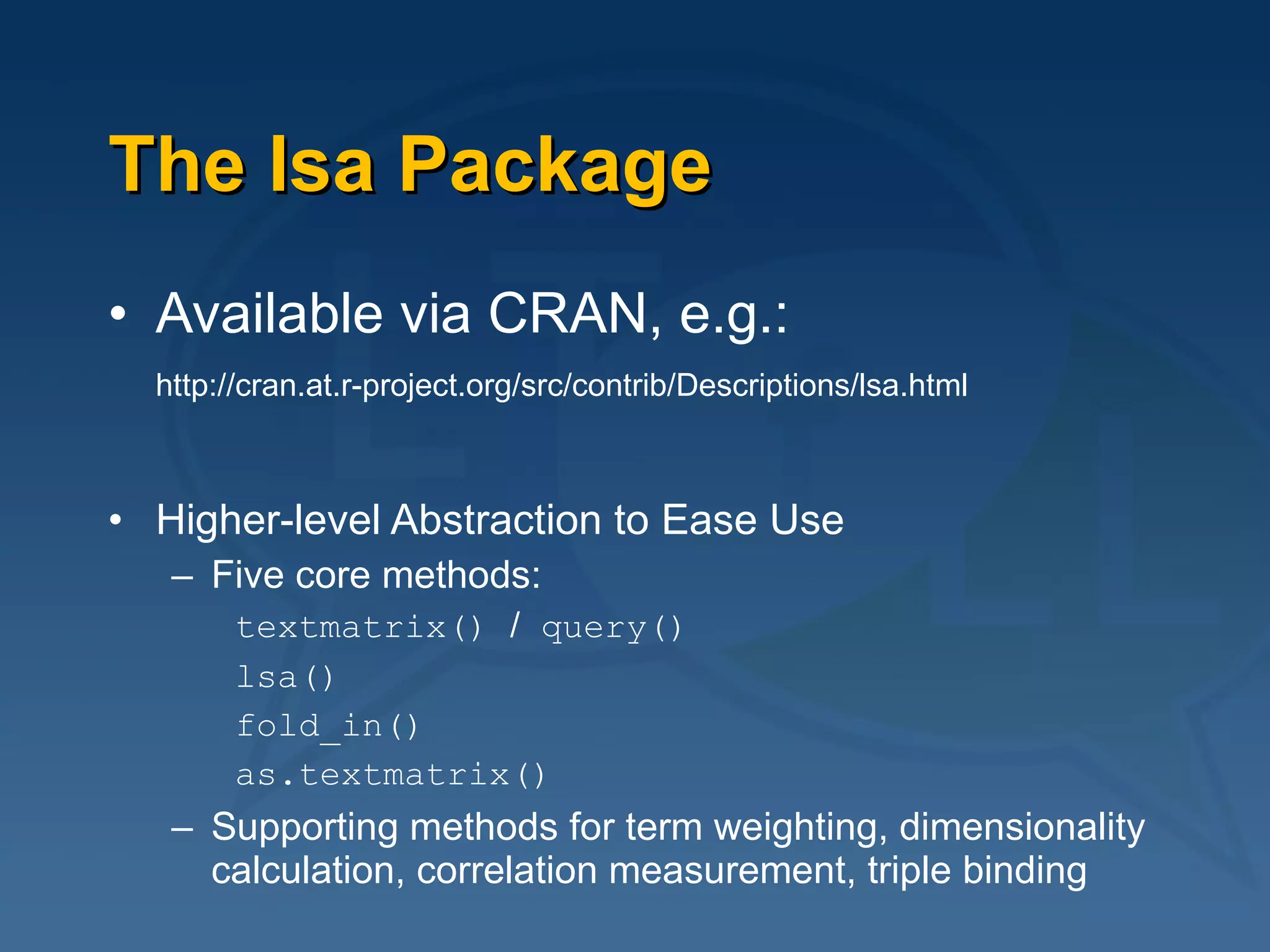

![How to do it... library( "lsa“ ) # load package # load training texts trm = textmatrix( "trainingtexts/“ ) trm = lw_bintf( trm ) * gw_idf( trm ) # weighting space = lsa( trm ) # create an LSA space # fold-in essays to be tested (including gold standard text) tem = textmatrix( "testessays/", vocabulary=rownames(trm) ) tem = lw_bintf( tem ) * gw_idf( trm ) # weighting tem_red = fold_in( tem, space ) # score an essay by comparing with # gold standard text (very simple method!) cor( tem_red[,"goldstandard.txt"], tem_red[,"E1.txt"] ) => 0.7](https://image.slidesharecdn.com/2009-06-04ltfllnlp-experiments-v2-090611044833-phpapp02/75/Language-Technology-Enhanced-Learning-22-2048.jpg)
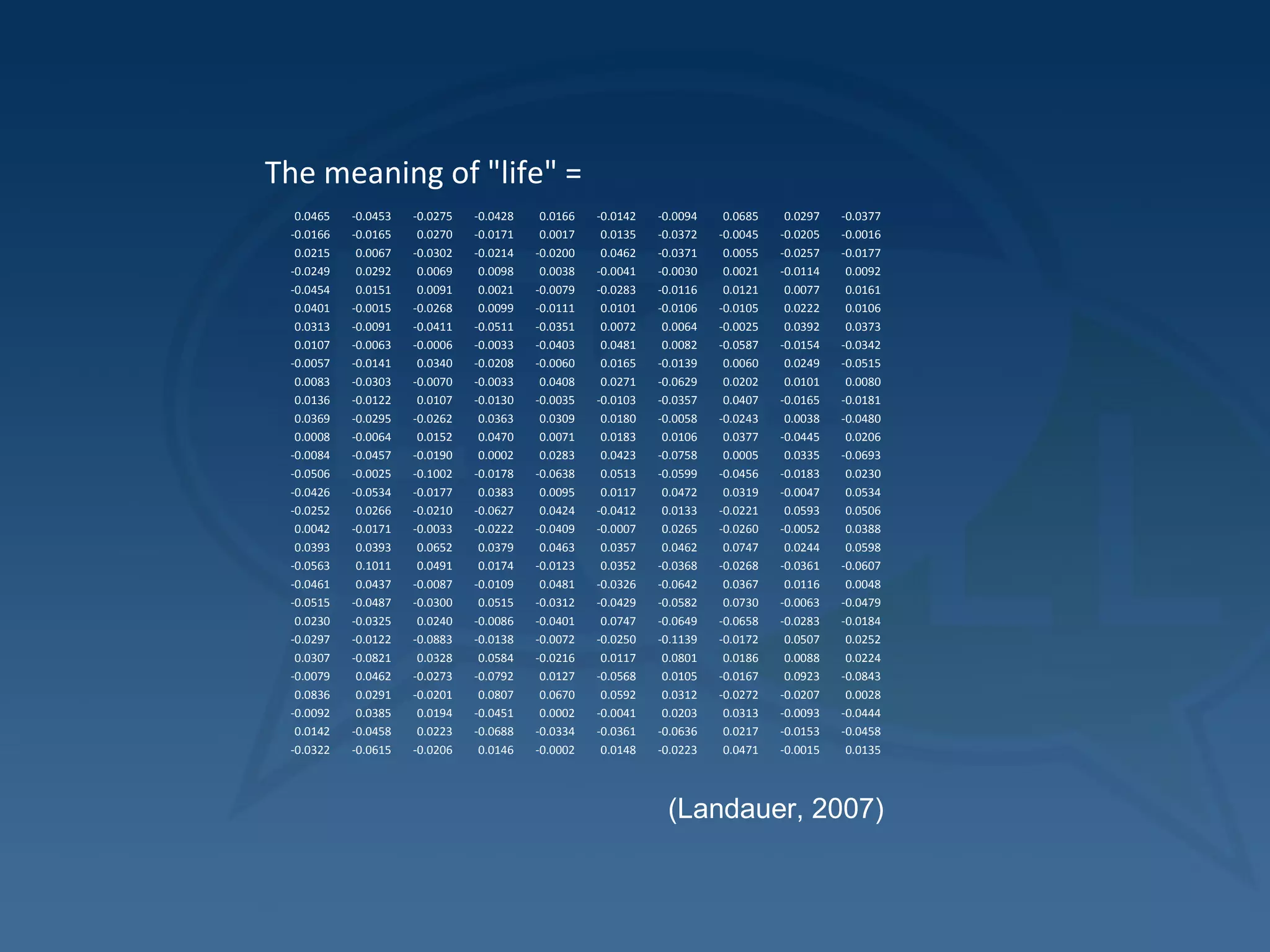
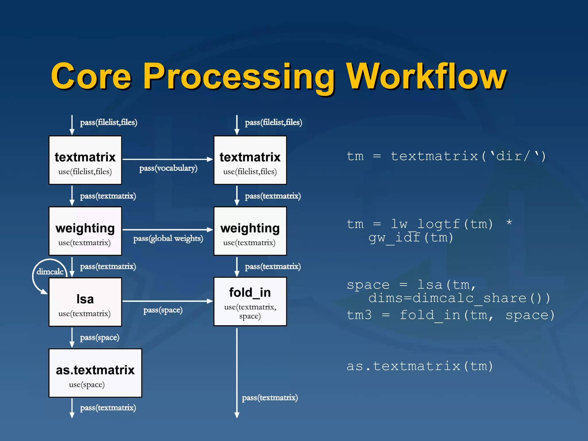
![(Positive) Evaluation Results LSA machine scores: Spearman's rank correlation rho data: humanscores[names(machinescores), ] and machinescores S = 914.5772, p-value = 0.0001049 alternative hypothesis: true rho is not equal to 0 sample estimates: rho 0.687324 Pure vector space model: Spearman's rank correlation rho data: humanscores[names(machinescores), ] and machinescores S = 1616.007, p-value = 0.02188 alternative hypothesis: true rho is not equal to 0 sample estimates: rho 0.4475188](https://image.slidesharecdn.com/2009-06-04ltfllnlp-experiments-v2-090611044833-phpapp02/75/Language-Technology-Enhanced-Learning-24-2048.jpg)

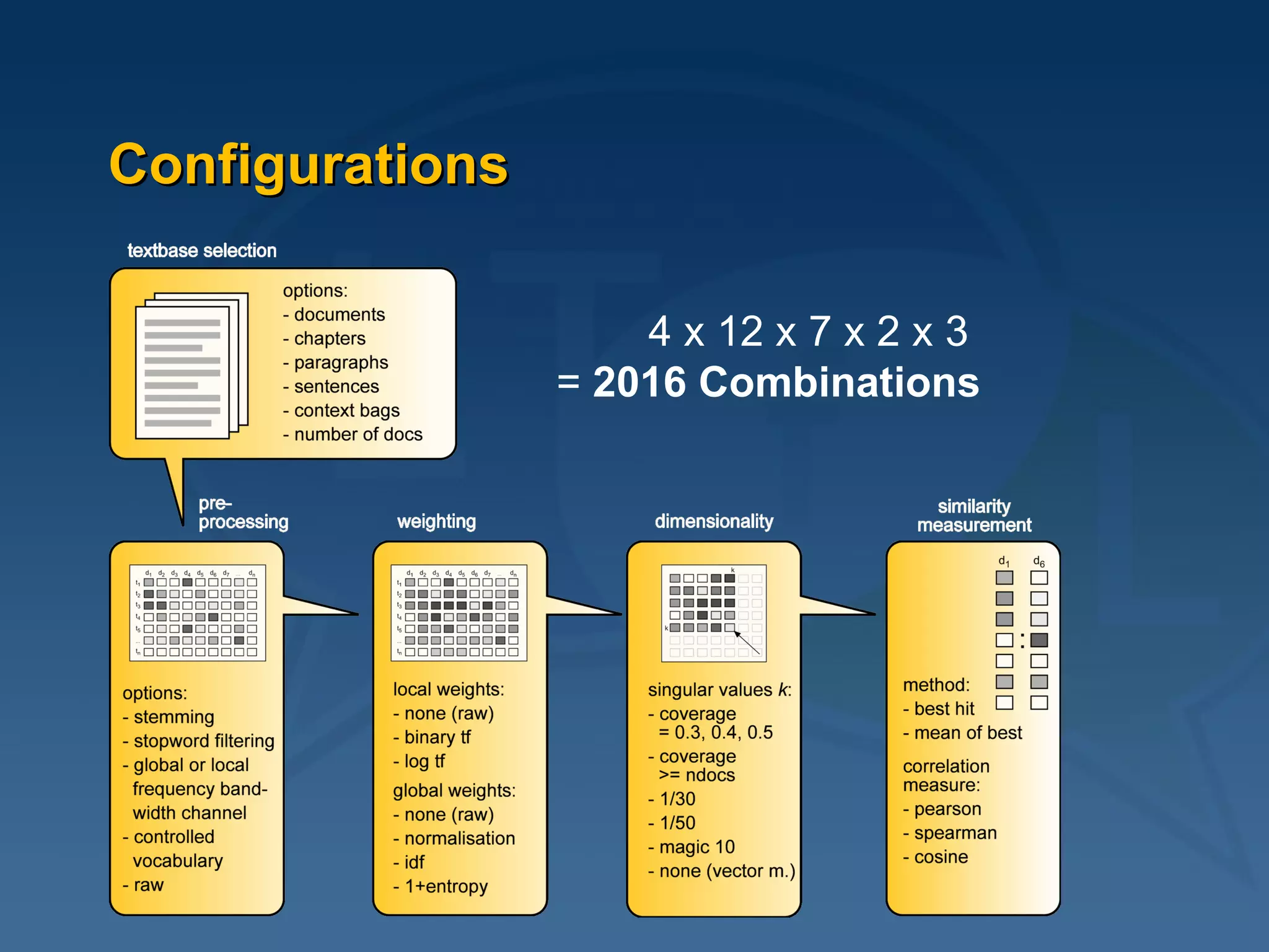
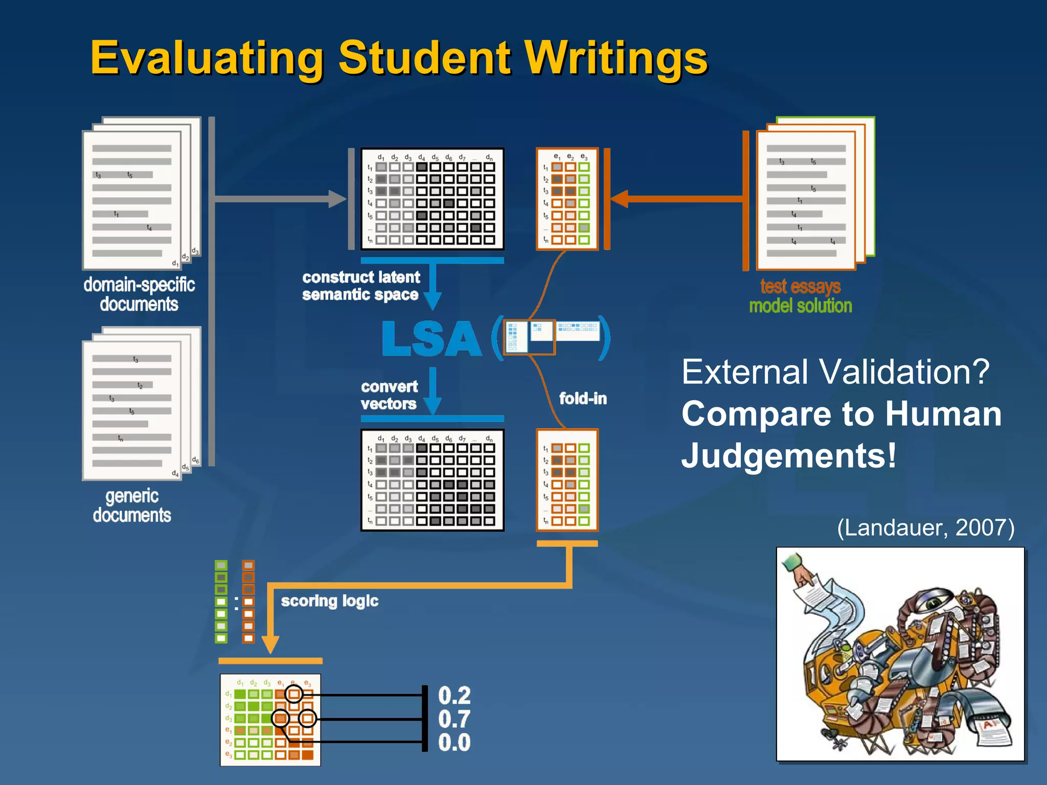
![Classical Landauer Example tl = landauerSpace$tk %*% diag(landauerSpace$sk) dl = landauerSpace$dk %*% diag(landauerSpace$sk) dtl = rbind(tl,dl) s = cosine(t(dtl)) s[which(s<0.8)] = 0 plot( network(s), displaylabels=T, vertex.col = c(rep(2,12), rep(3,9)) )](https://image.slidesharecdn.com/2009-06-04ltfllnlp-experiments-v2-090611044833-phpapp02/75/Language-Technology-Enhanced-Learning-28-2048.jpg)
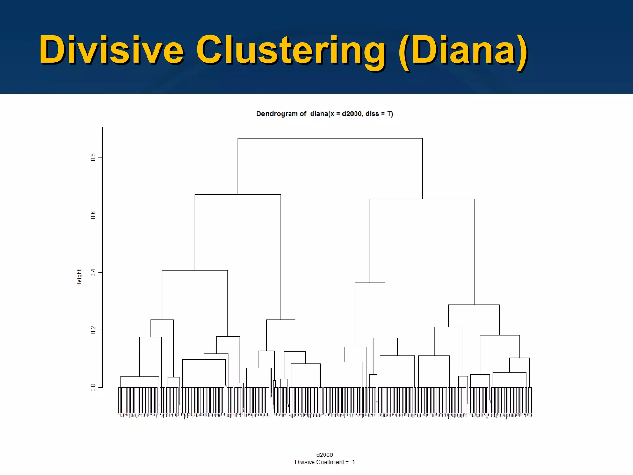
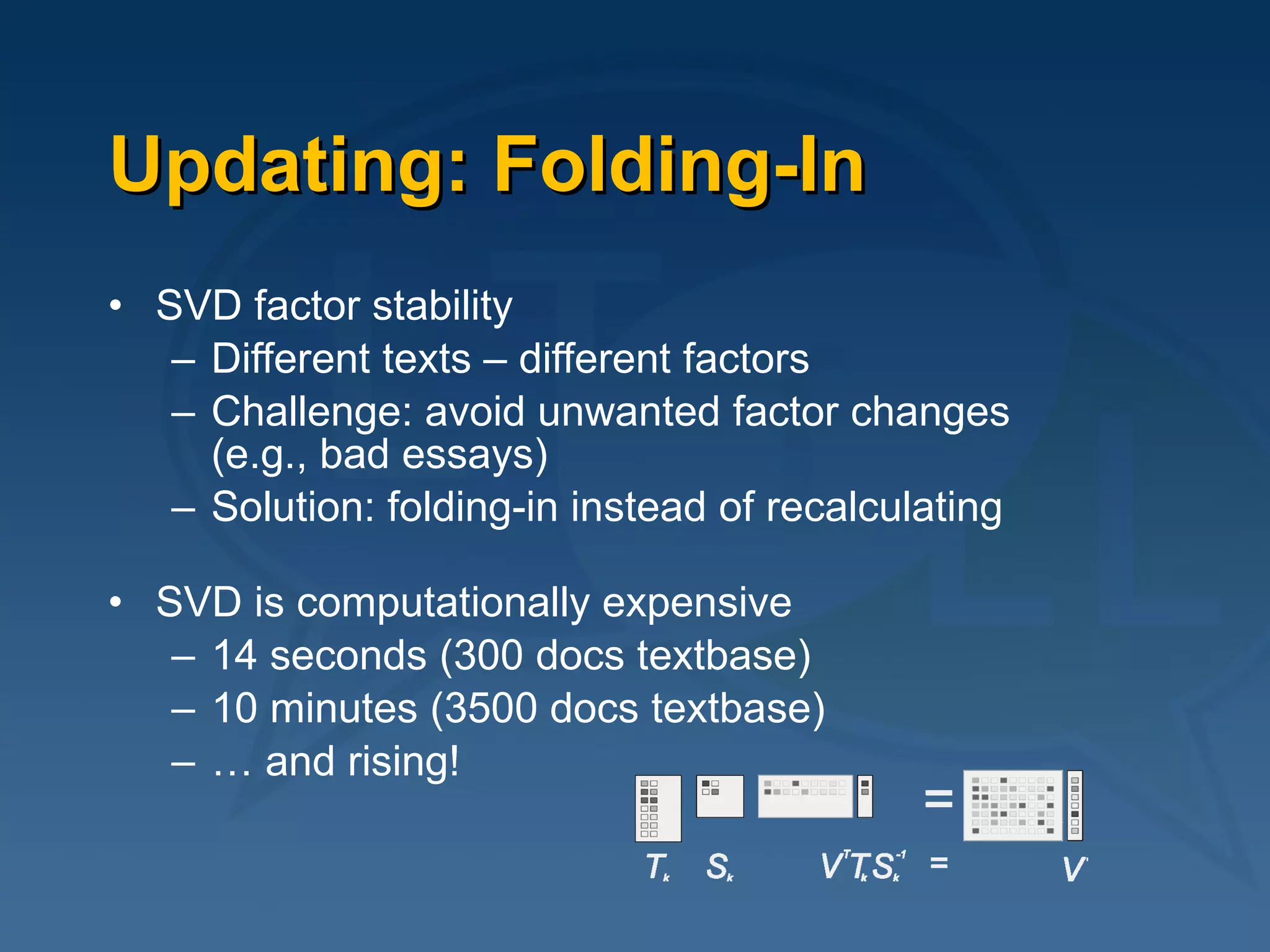
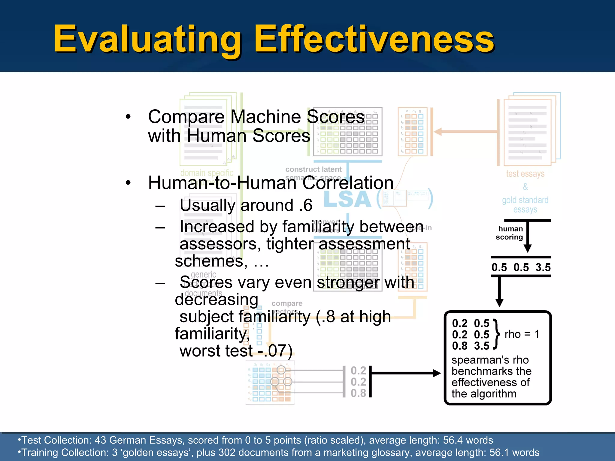
![Code Sample d2000 = cosine(t(dtm2000)) dianac2000 = diana(d2000, diss=T) clustersc2000 = cutree(as.hclust(dianac2000), h=0.2) plot(dianac2000, which.plot=2, cex=.1) # dendrogramme winc = clustersc2000[which(clustersc2000==1)] # filter for cluster 1 wincn = names(winc) d = d2000[wincn,wincn] d[which(d<0)] == 0 btw = betweenness(d, cmode="undirected") # for nodes size calc btwmax = colnames(d)[which(btw==max(btw))] btwcex = (btw/max(btw))+1 plot(network(d), displayisolates=F, displaylabels=T, boxed.labels=F, edge.col="gray", main=paste("cluster",i), usearrows=F, vertex.border="darkgray", label.col="darkgray", vertex.cex=btwcex*3, vertex.col=8-(colnames(d) %in% btwmax))](https://image.slidesharecdn.com/2009-06-04ltfllnlp-experiments-v2-090611044833-phpapp02/75/Language-Technology-Enhanced-Learning-31-2048.jpg)


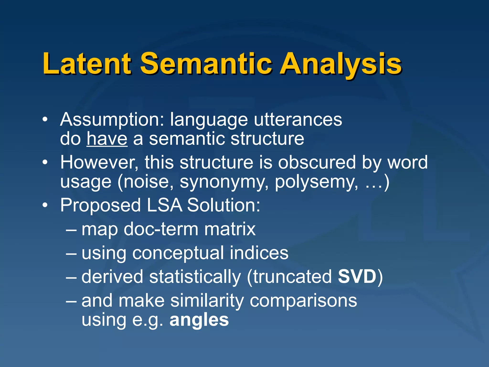
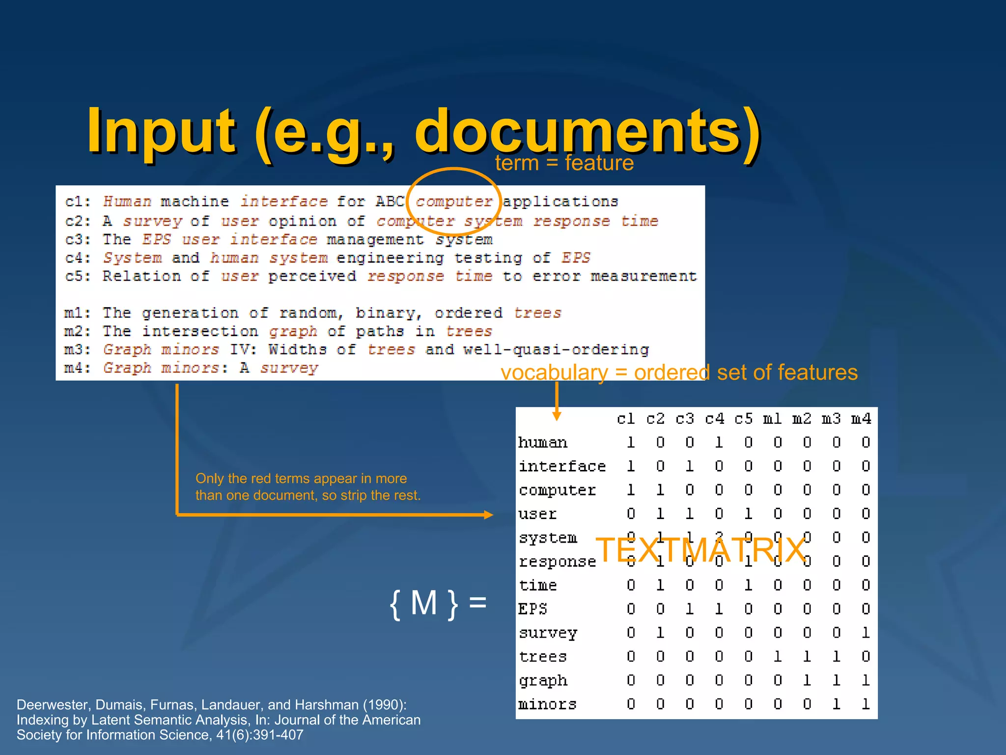
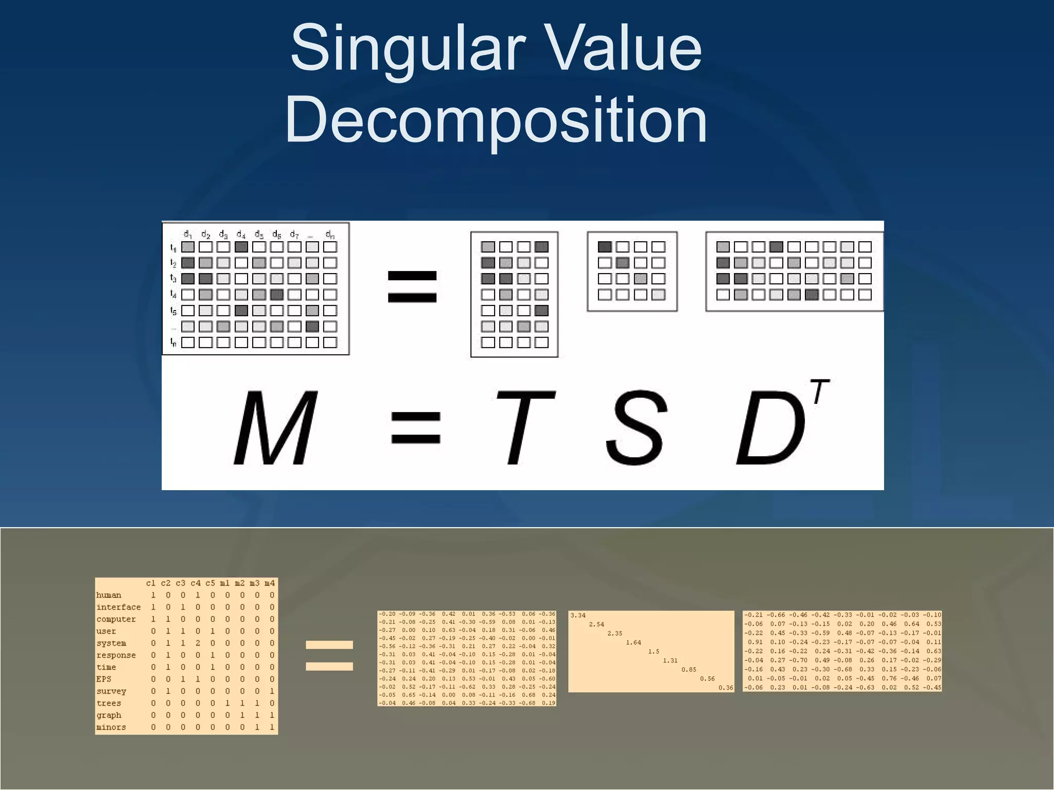
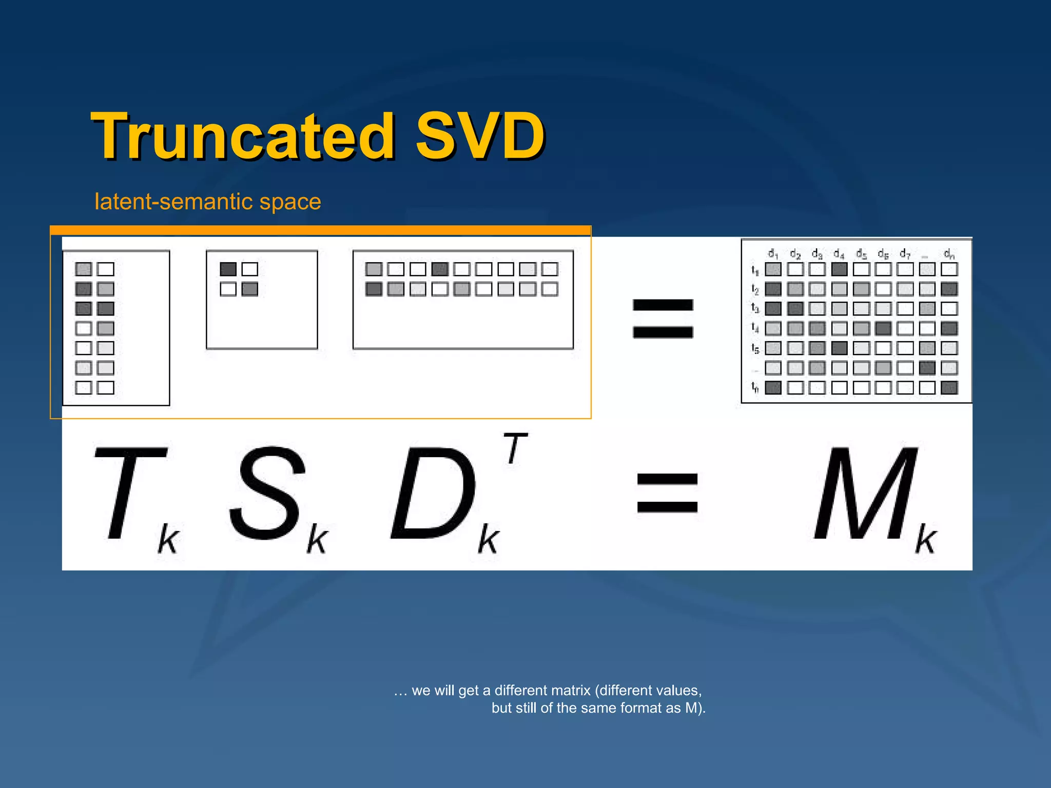
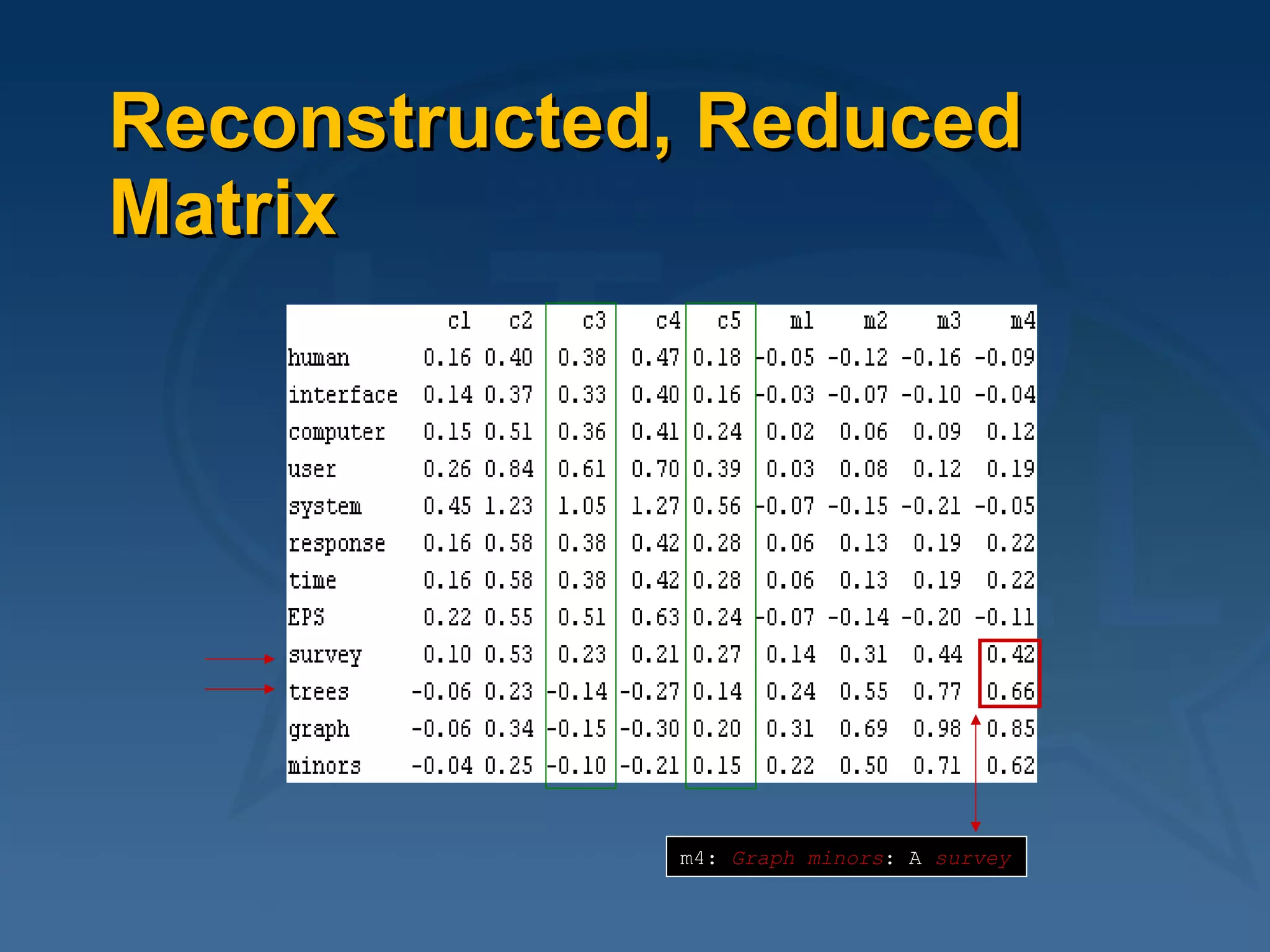
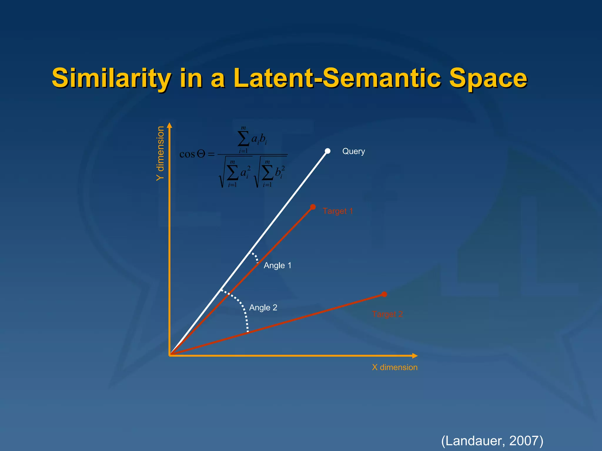
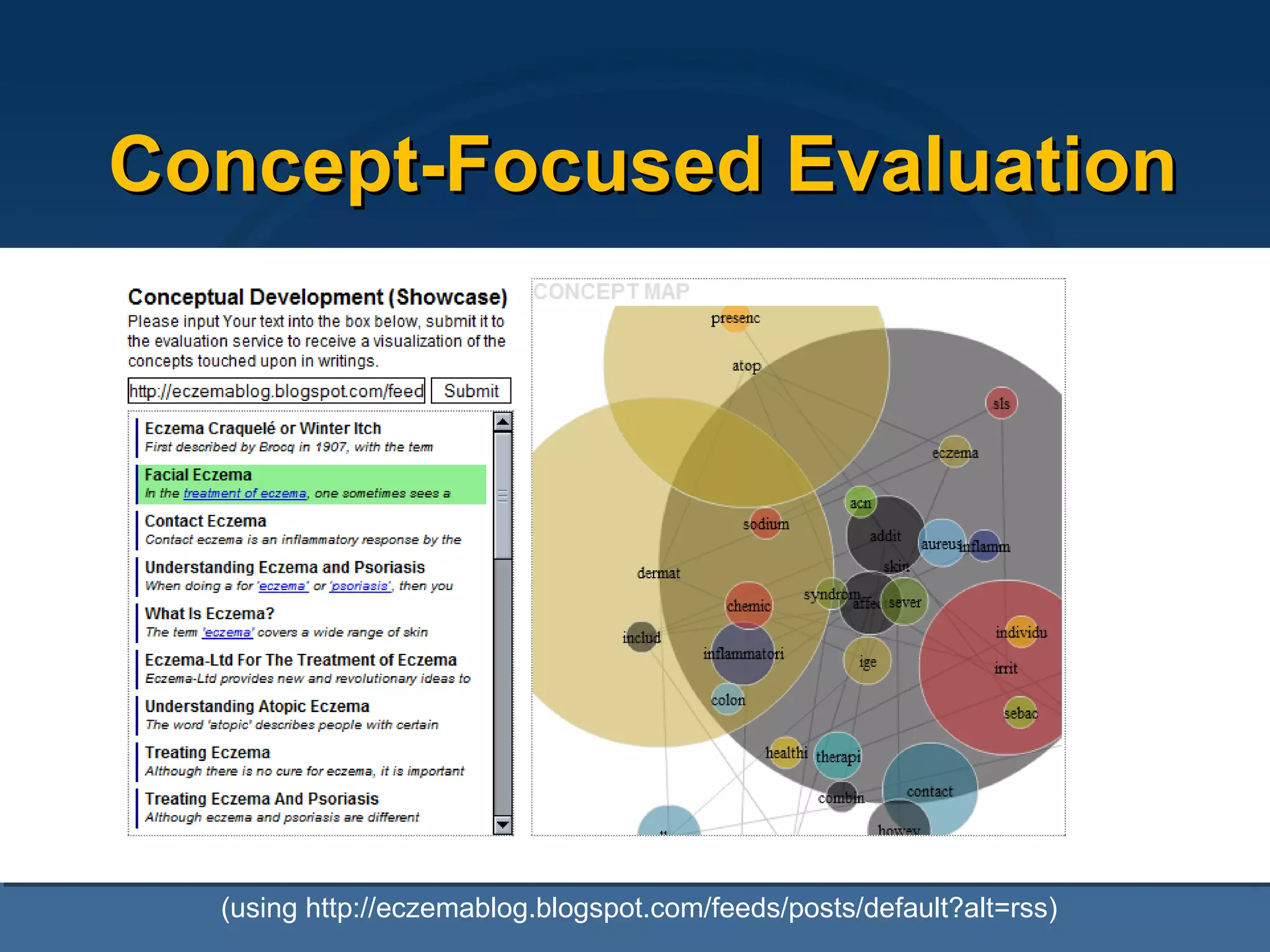
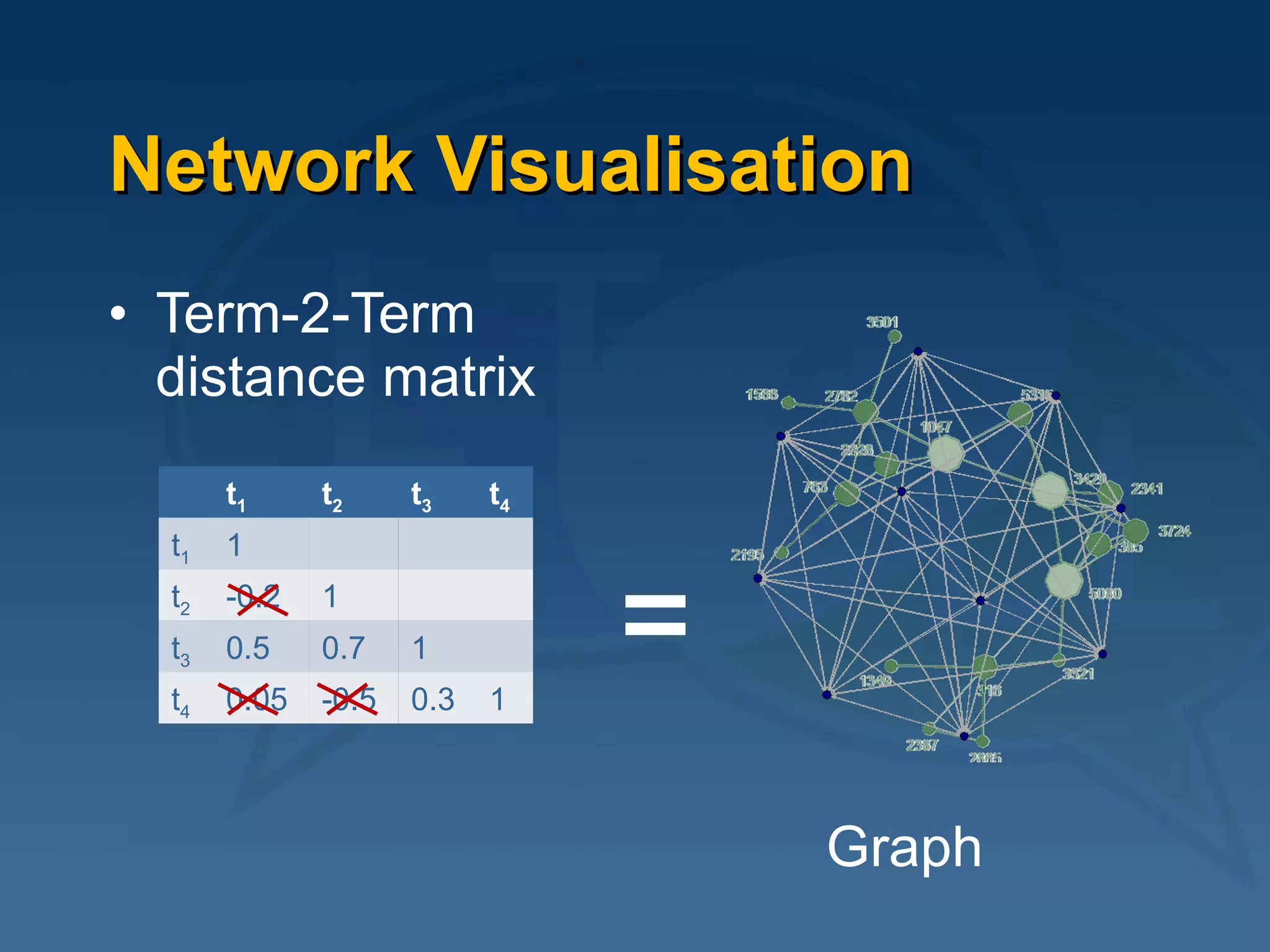
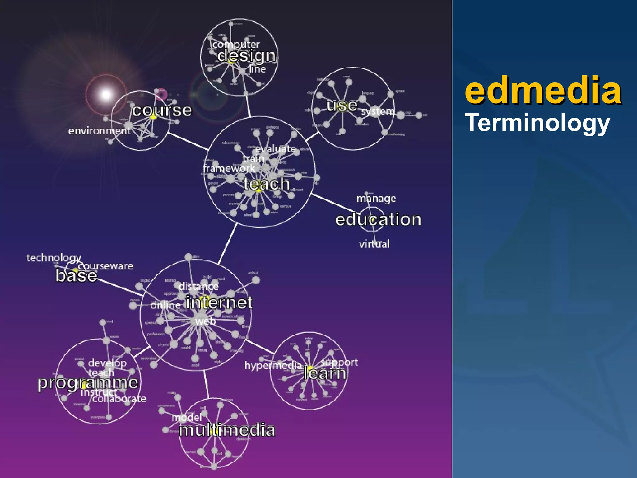
This document provides an overview of using latent semantic analysis (LSA) and the R programming language for language technology enhanced learning applications. It describes using LSA to create a semantic space to compare documents and evaluate student writings. It also demonstrates clustering terms based on their semantic similarity and visualizing networks in R. Evaluation results show LSA machine scores for essay quality had a Spearman's rank correlation of 0.687 with human scores, outperforming a pure vector space model.