Slip line field method and its application in forming process Final year project work for Manufacturing Process class

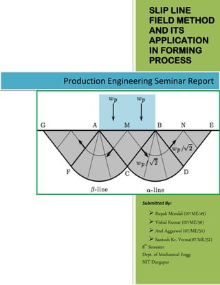
1. SLIP LINE
FIELD METHOD
AND ITS
APPLICATION
IN FORMING
PROCESS
Submitted By:
 Rupak Mondal (07/ME/49)
 Vishal Kumar (07/ME/50)
 Atul Aggarwal (07/ME/51)
 Santosh Kr. Verma(07/ME/52)
8th
Semester
Dept. of Mechanical Engg.
NIT Durgapur
Production Engineering Seminar Report

2. TABLE OF CONTENTS
Page
NOMENCLATURE............................................................................................1
INTRODUCTION...............................................................................................2
What Is Slip……………………………………...................................................................................2
Slip Line Field Method………………………….............................................................................2
Assumptions……………………..................................................................................................3
Slip Lines………………………………………....................................................................................5
Boundary Conditions..........................................................................................................5
SIGNIFICANCE…………………………………………………………..………………………..6
Advantages Of Slip Line Field Method................................................................................6
Limitations Of Slip Line Field Method.................................................................................6
Stress State At A Point In The Slip Line Field.......................................................................7
EXAMPLE SHOWING USE OF SLIP LINE FIELD METHOD IN
FORMING PROCESS …………………………………….……………………………………8
Uniaxial Tension……………………………………………………………………………………………………………..8
Plane Strain Extrusion (Hill)…………………………………………………………………………………………….9
Double Notched Plate In Tension.....................................................................................10
REFERENCES……………………………………………………………………………………11

3. NOMENCLATURE
bf the flash land width
Δbf, Δhb displacement of the free surface of boss and the free surface
of flash in one stage of simulation
Bb the boss width
d the forging width
F load
g thickness of the forging
Δhd displacement of the mobile die in one stage of simulation
hf thickness of the flash land
H height of the forging (without the boss)
Hb the boss height
k the yield stress in pure shear
m friction factor
n number of iterations in the simulation
p mean pressure (stress)
vd, vb,vf velocity of the mobile die, the free surface of boss and the
free surface of the flash
wp ratio of the velocity
α, β slip-lines (principal shear stress direction)
Γ the poly-optimal function
θ draft angle in the forging
σ, τ stress component
ϕ the angle of inclination of the α-principal shear stress
direction measured in the anticlockwise direction from the x-
axis
χ coefficient of the poly-optimal function

4. INTRODUCTION
What Is Slip?
The process which allows plastic flow to occur in metals, where the crystal
planes slide past one another. In practice, the force needed for the entire
block of crystal to slide is very great, and so the movement occurs by
dislocation motion along the slip planes, which requires much lower level
of stress.
Slip Line Field Method
The slip-line field analysis, a graphical approach, depends upon the
determination of the plastic flow pattern in the deforming material. Plastic
flow, as discussed earlier, occurs predominantly by slip on planes of closely
packed atoms and in the direction of the line of atoms which lie closest to the
line of maximum shear stress. In a real material, it is reasonable to assume
that there will be sufficient number of favourably oriented planes for the slip
direction to coincide with the direction of maximum shear stress. In an ideal
material, i.e., a structure less, homogeneous and isotropic material, the slip
will always occur precisely in the direction of maximum shear stress. Thus,
once the direction of maximum shear stress is known, the direction of plastic
flow in an ideal material is known.
In a deforming material the planes of maximum shear stress form an
orthogonal curvilinear network as shown in the figure below. These
orthogonal networks of the lines of maximum shear stress have come to be
known as the slip-line field and the directions of maximum shear stress as
the slip lines.

5. The general direction of three-dimensional deformation is still intractable,
but it is possible to analyze a plane strain situation, the strain in the
direction of the third principal strain is zero.
Assumptions
This theory simplifies the governing equations for plastic deformation by
making several assumptions:
a. Rigid-Plastic Material Response: - A rigid-plastic material is defined as
a material exhibiting no elastic deformation and perfect plastic
deformation. Compared to a real metal, all elastic behaviour and strain
hardening effects are ignored.
Fig 1. Rigid Plastic Material Response
b. Plane strain deformation: - Much deformation of practical interest
occurs under a condition that is nearly, if not exactly, one of plane
strain, i.e. where one principal strain (say ε3) is zero so that δε3=0.

6. Plane strain is applicable to rolling, drawing and forging where flow in
a particular direction is constrained by the geometry of the machinery,
e.g. a well-lubricated die wall.
A specific example of this is in rolling, where the major deformation
occurs perpendicular to the roll axis. The material becomes thinner
and longer but not wider. Frictional stresses parallel to the rolls (i.e. in
the width direction) prevent deformation in this direction and hence a
plane strain condition is produced where δε3=0.
Plane strain condition in plastic deformation
From Tresca and von Mises yield criteria, we find:
 Tresca (k = shear yield stress and Y = uniaxial yield
stress)
 von Mises
If
Therefore, if we have plane strain, the Tresca yield criterion and
the von Mises yield criterion have the same result expressed in
terms of k. It is unnecessary to specify which criterion we are
using, provided we use k.
c. Quasi-static loading: - A static load is time independent. A dynamic
load is time dependent and for which inertial effects cannot be ignored.
A quasi-static load is time dependent but is "slow" enough such that
inertial effects can be ignored. Note that load quasi-static for a given
structure (made of some material) may not be quasi-static for another
structure (made of a different material).
d. No temperature change and no body force;
e. Isotropic material: - Isotropic materials are characterized by properties
which are independent of direction in space. Physical equations
involving isotropic materials must therefore be independent of the
coordinate system chosen to represent them.
f. No work hardening

7. Slip Lines
The two directions of maximum shear stresses or the slip-lines are usually
identified α and β-lines. The usual convention for identifying is that when α
and β-lines from a right handed co-ordinate system of axes, then the direction
of the algebraically greatest principal stress lies in the third quadrant.
Boundary Conditions
One can always determine the direction of one principal stress at a boundary.
The following boundary conditions are useful:
1) The force and stress normal to a free surface is a principal stress, so the α
and β -lines must meet the surface at 450.
2) The α and β -lines must meet a frictionless surface at 450.
3) The α and β -lines meet surfaces of sticking friction at 00 and 900.

8. SIGNIFICANCE
This approach is used to model plastic deformation in plane strain only for a
solid that can be represented as a rigid-plastic body. Elasticity is not included
and the loading has to be quasi-static. In terms of applications, the approach
now has been largely superseded by finite element modeling, as this is not
constrained in the same way and for which there are now many commercial
packages designed for complex loading (including static and dynamic forces
plus temperature variations). Nonetheless, slip line field theory can provide
analytical solutions to a number of metal forming processes, and utilizes plots
showing the directions of maximum shear stress in a rigid-plastic body which
is deforming plastically in plane strain. These plots show anticipated
patterns of plastic deformation from which the resulting stress and strain
fields can be estimated.
1. Advantages of slip line field method:
Because of huge deformation and velocity discontinuities, numerical solutions
are not possible and then analytical solutions are used.
2. Limitations of slip line field method:
It is very harder to implement and use in comparison to FEM package.

9. Stress state at a point in the slip-line field
By definition, the slip-lines are always parallel to axes of principal shear
stress in the solid. This means that the stress components in a basis oriented
with the , directions have the form
where is the hydrostatic
stress (determined using the equations given below), k is the yield stress of
the material in shear, and Y is its yield stress in uniaxial tension. This stress
state is sketched in the figure. Since the shear stress is equal to the shear
yield stress, the material evidently deforms by shearing parallel to the slip-
lines: this is the reason for their name.
If denotes the angle between the slip-line and the direction, the stress
components in the basis can be calculated as
The Mohr’s circle construction (shown in the picture to the right) is a
convenient way to remember these results.
x
 k k 

e1
e2
 slip-line

dy/dx = tan
dy/dx = -cot
e
 slip-line
e 




k 

10. EXAMPLE SHOWING USE OF SLIP LINE
FIELD METHOD IN FORMING PROCESS
1. Uniaxial Tension
We can easily see that the slip lines are along 450 and -450 directions, which
is straightforward by using Mohr’s circle. Consider tension in two 1 and 2
directions,
Also, slip lines are along 450 and -450 directions because the present
configuration is just the superposition of two uniaxial tensions.

11. 2. Plane Strain Extrusion (Hill)
A slip-line field solution to plane strain extrusion through a tapered die is
shown in the picture on the right. Friction between the die and work piece is
neglected.
It is of particular interest to calculate the force P required to extrude the bar.
The easiest way to do this is to consider the forces acting on the region
ABCDEF. Note that
 The resultant force on EF is
 The resultant force on CB is zero (you can see this by noting that no
external forces act on the material to the left of CB)
 The stress state at a point b on the line CD can be calculated by
tracing a slip-line from a to b. The Mohr’s circle construction for this
purpose is shown on the right. At point a, the slip-lines intersect CB at
45 degrees, so that ; we also know that on CB (because
the solid to the left of CB has no forces acting on it). These conditions
can be satisfied by choosing , so that the stress state at a is
. Tracing a slip-line from a to b, we see that
. Finally, the slip lines intersect CD at 45
degrees, so CD is subjected to a pressure acting normal to
CD, while the component of traction tangent to CD is zero.
 CD has length H, so the resultant force acting on CD is
 By symmetry, the resultant force acting on AB is
 Equilibrium then gives

slip-line
slip-line

H 2H
30o
45o
45o
P
A
B
C
D
a
b E
F
e1
e2




k

k
k
nn
ab


12. 3. Rigid Punch Indenting a Plastic Solid
Here Hill’s problem of a rigid punch indenting a plastic solid has been
considered to find the load P that allows the punch to indent into the plastic
solid.
At point a, φa=450
At point a, φa=450
@point a:
@point b:
( )
( )
The pressure under the punch turns out to be uniform, so integral
of over the area should balance the applied force P,
√
,w is the width of the punch.

13. 4. Double-Notched Plate In Tension
A slip-line field solution for a double-notched plate under tensile loading is
shown in the picture. The stress state in the neck, and the load P are of
particular interest.
Both can be found by tracing a slip-line from either boundary into the
constant stress region at the center of the solid.
Consider the slip-line starting at A and ending at B, for example. At A the
slip-lines meet the free surface at 45 degrees. With designated as shown,
and . Following the slip-line to b, we see that , so
the Hencky equation gives . The state of stress at b follows as
The state of stress is clearly constant in the region ABCD, (and so is constant
along the line connecting the two notches). The force required to deform the
solid is therefore .
 slip-line slip-line

P
P

a
A
B

14. REFERENCES
1. G K Lal , Introduction to Machining Science.
2. http://solidmechanics.org/text/Chapter6_1/Chapter6_1.htm
3. http://www.engin.brown.edu/courses/en222/Notes/sliplines/sliplines.htm
4. http://www.globalspec.com/reference/70308/203279/html-head-chapter-9-
slip-line-field-analysis