Downloaded 390 times
![ Variance of a discrete random variable
Standard Deviation of a discrete random variable
where:
E(X) = Expected value of the discrete random variable X
Xi = the ith
outcome of X
P(Xi) = Probability of the ith
occurrence of X
Discrete Random Variables
Measuring Dispersion
∑=
−=
N
1i
i
2
i
2
)P(XE(X)][Xσ
∑=
−==
N
1i
i
2
i
2
)P(XE(X)][Xσσ](https://image.slidesharecdn.com/probabilitydistribution2-150117052555-conversion-gate01/75/Probability-distribution-2-8-2048.jpg)
![ Example: Toss 2 coins, X = # heads,
compute standard deviation (recall E(X) = 1)
Discrete Random Variables
Measuring Dispersion
)P(XE(X)][Xσ i
2
i
−= ∑
0.7070.50(0.25)1)(2(0.50)1)(1(0.25)1)(0σ 222
==−+−+−=
(continued)
Possible number of heads
= 0, 1, or 2](https://image.slidesharecdn.com/probabilitydistribution2-150117052555-conversion-gate01/75/Probability-distribution-2-9-2048.jpg)
![The Covariance Formula
The covariance formula:
)YX(P)]Y(EY)][(X(EX[σ
N
1i
iiiiXY ∑=
−−=
where: X = discrete random variable X
Xi = the ith
outcome of X
Y = discrete random variable Y
Yi = the ith
outcome of Y
P(XiYi) = probability of occurrence of the
ith
outcome of X and the ith
outcome of Y](https://image.slidesharecdn.com/probabilitydistribution2-150117052555-conversion-gate01/75/Probability-distribution-2-11-2048.jpg)

This document defines discrete and continuous random variables and provides examples of each. It then focuses on discrete random variables and probability distributions. Specifically, it discusses the binomial probability distribution, giving its formula and providing examples of calculating binomial probabilities. It also discusses properties of the binomial distribution such as its shape and mean, and shows how binomial tables can be used to find probabilities.
Introduction to discrete probability distributions and definitions of random variables.
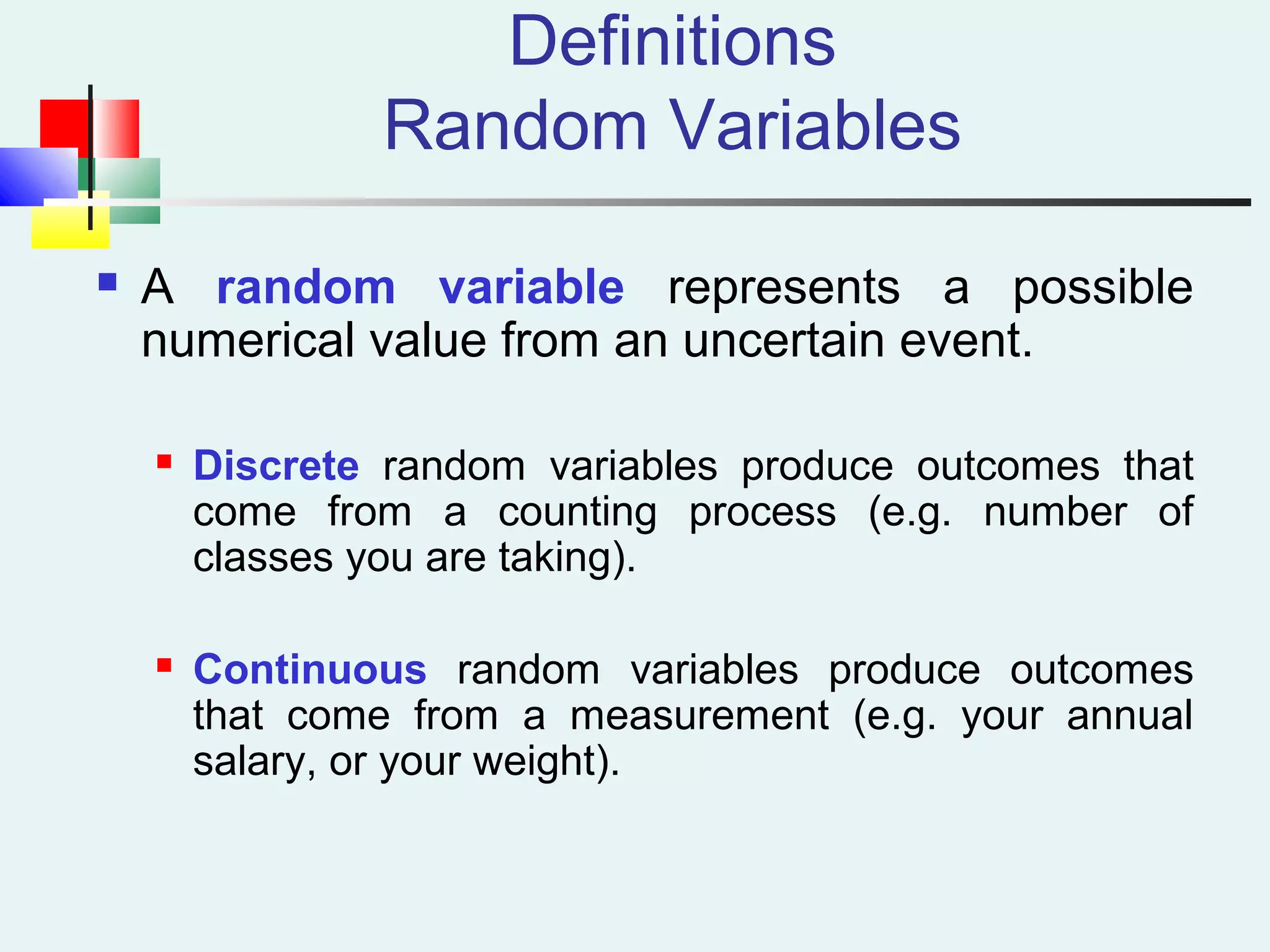
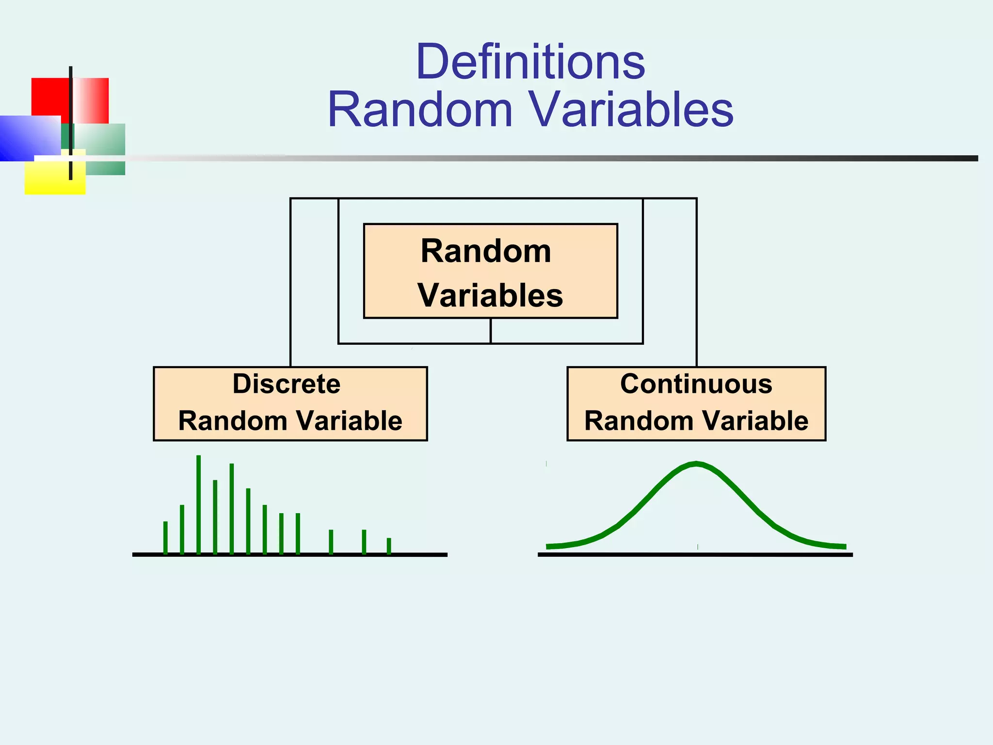
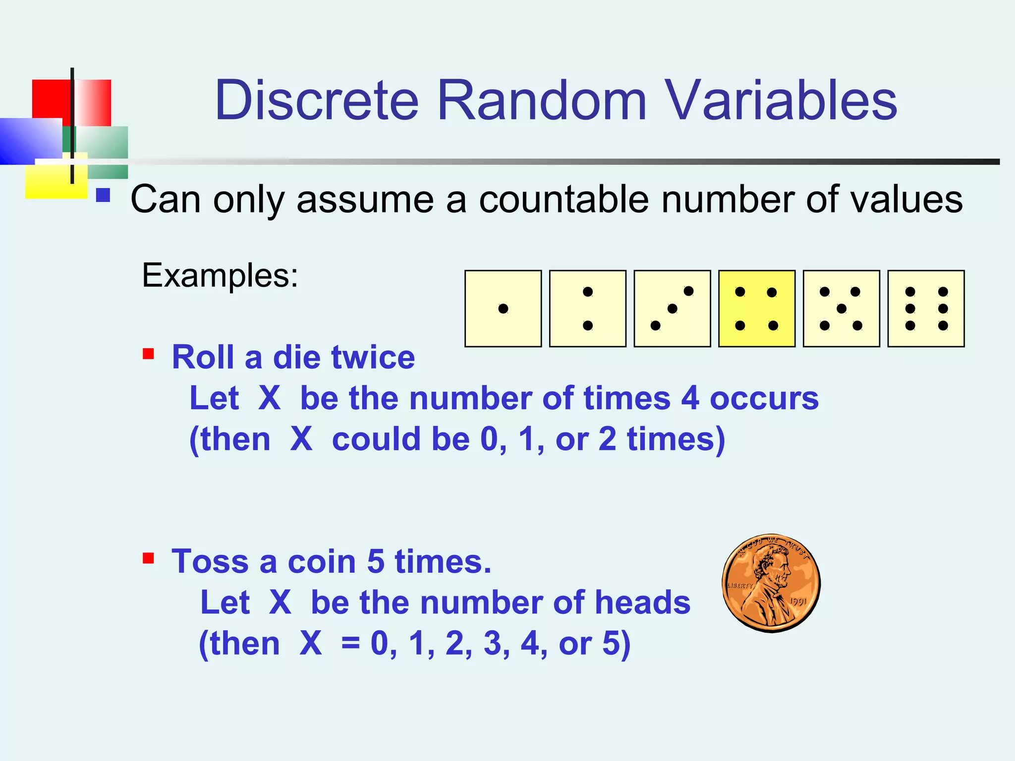
Focus on types of random variables: discrete and continuous, with examples like die rolls and coin tosses.
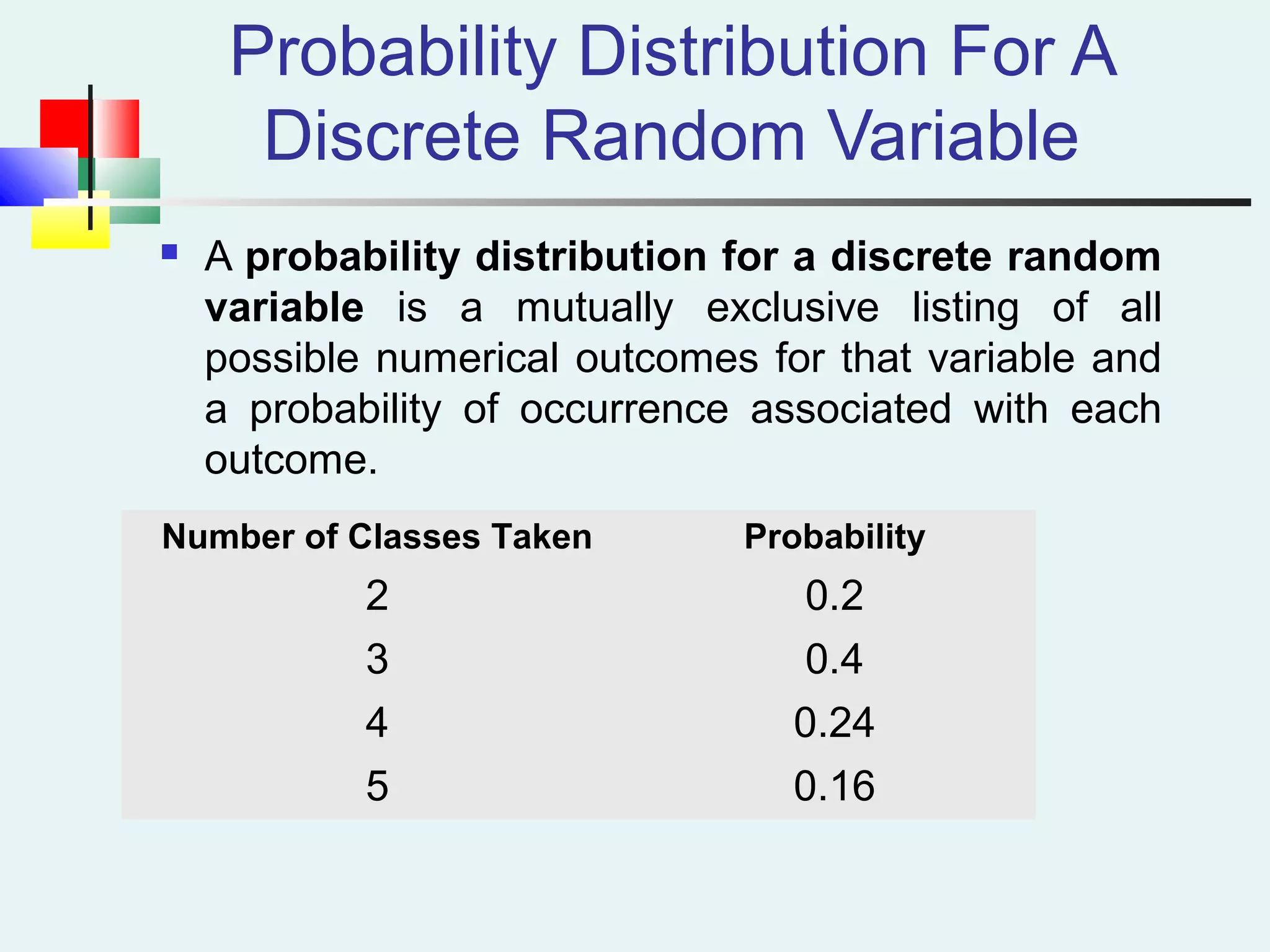
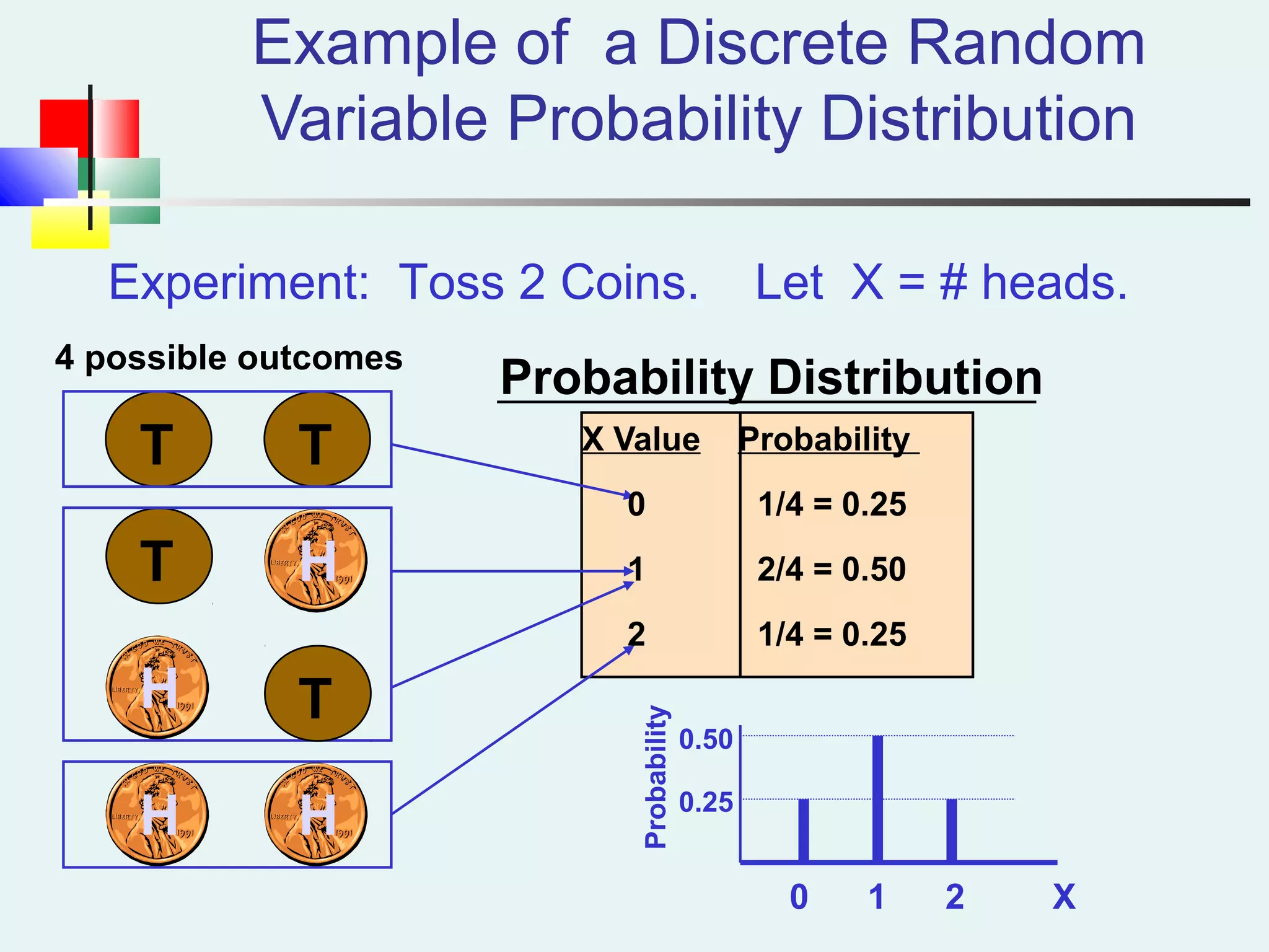
Explanation of probability distributions for discrete random variables with numerical outcomes.
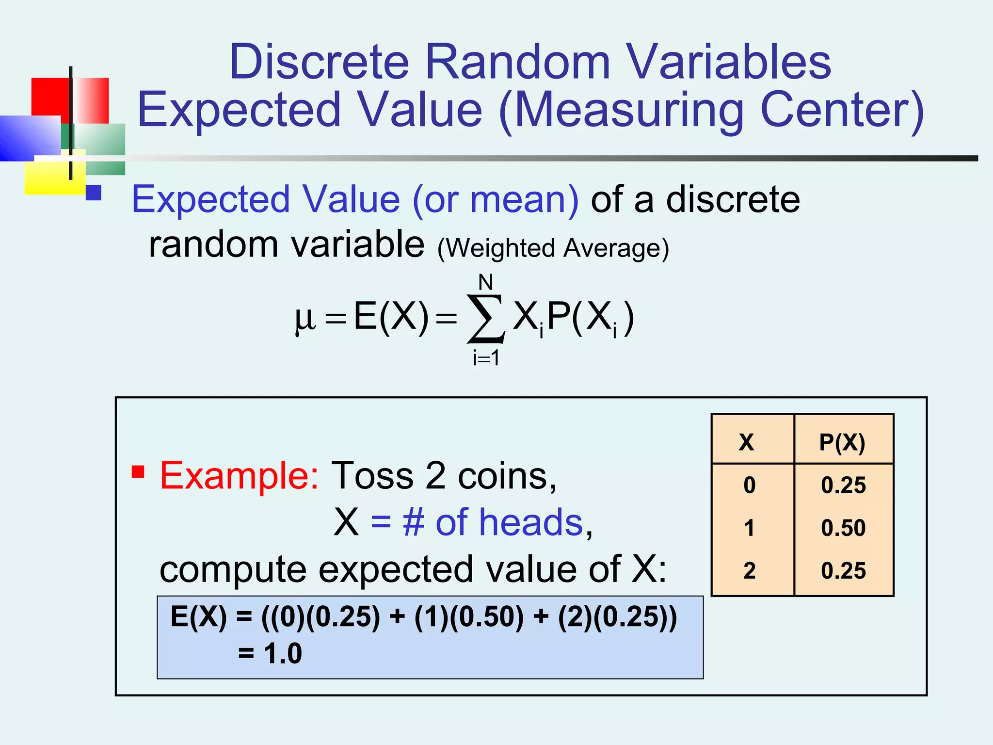
Explains expected value, variance, and standard deviation for discrete random variables with examples.
Introduction to covariance, measuring relationships between discrete random variables.
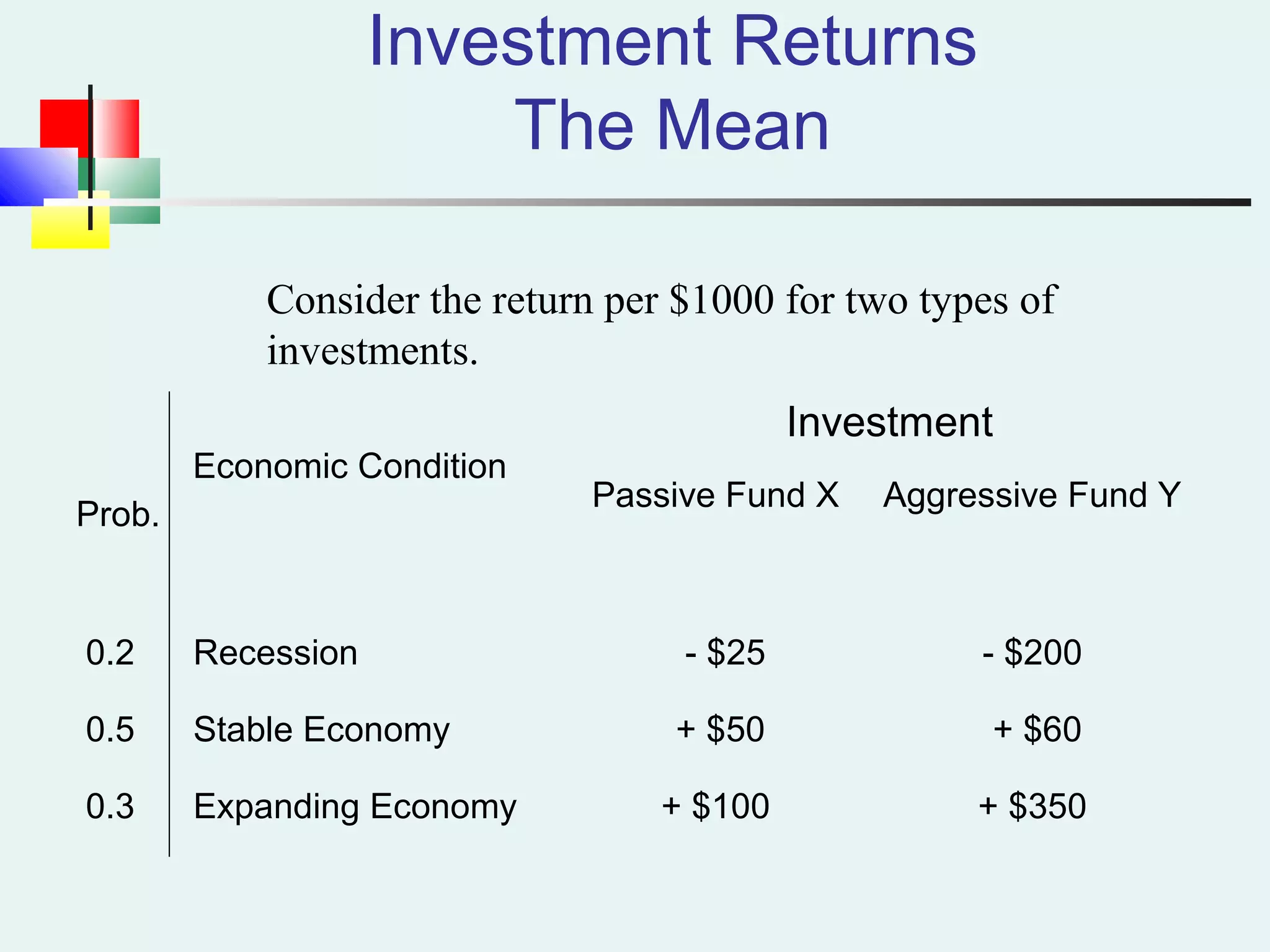
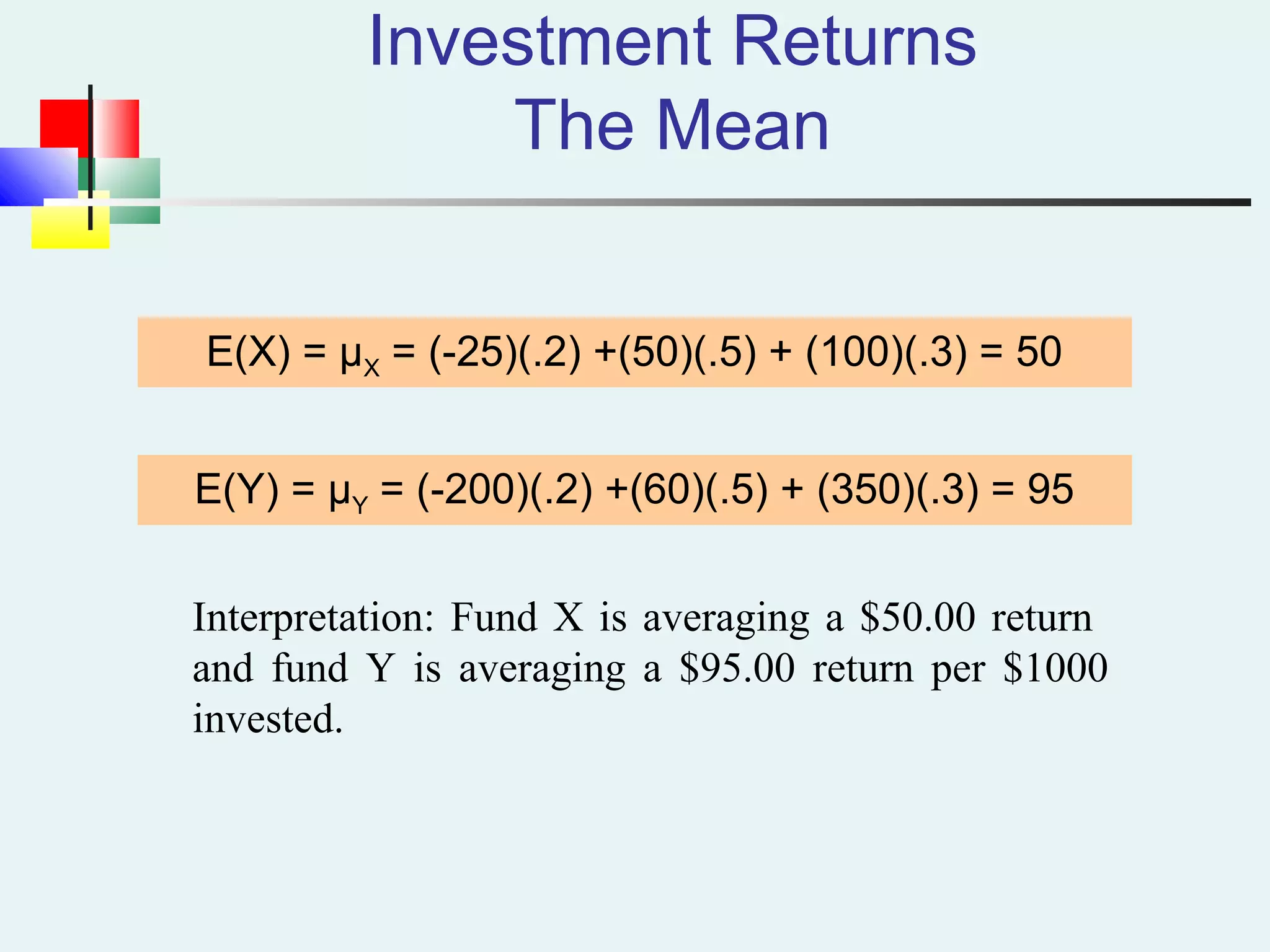
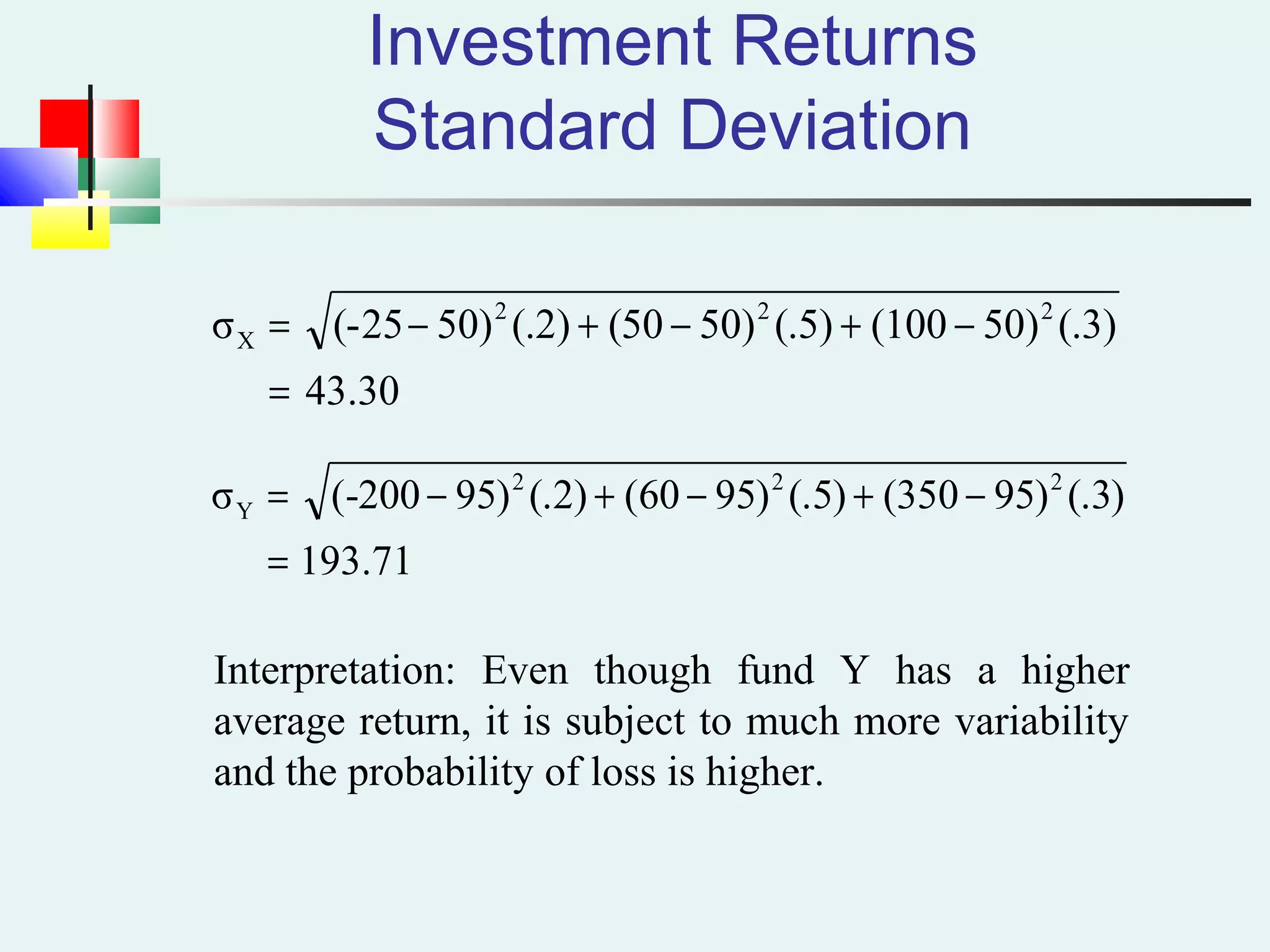
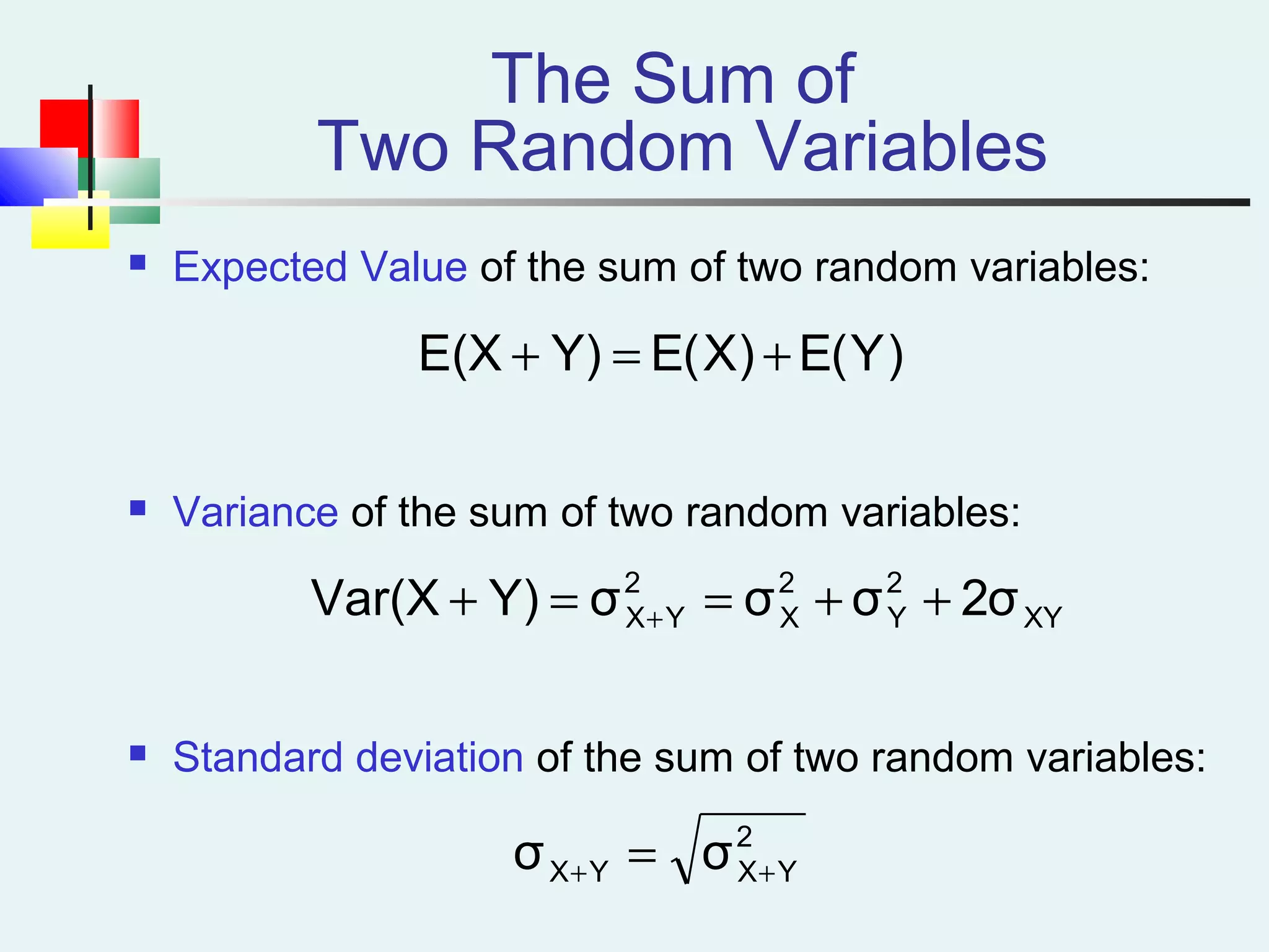
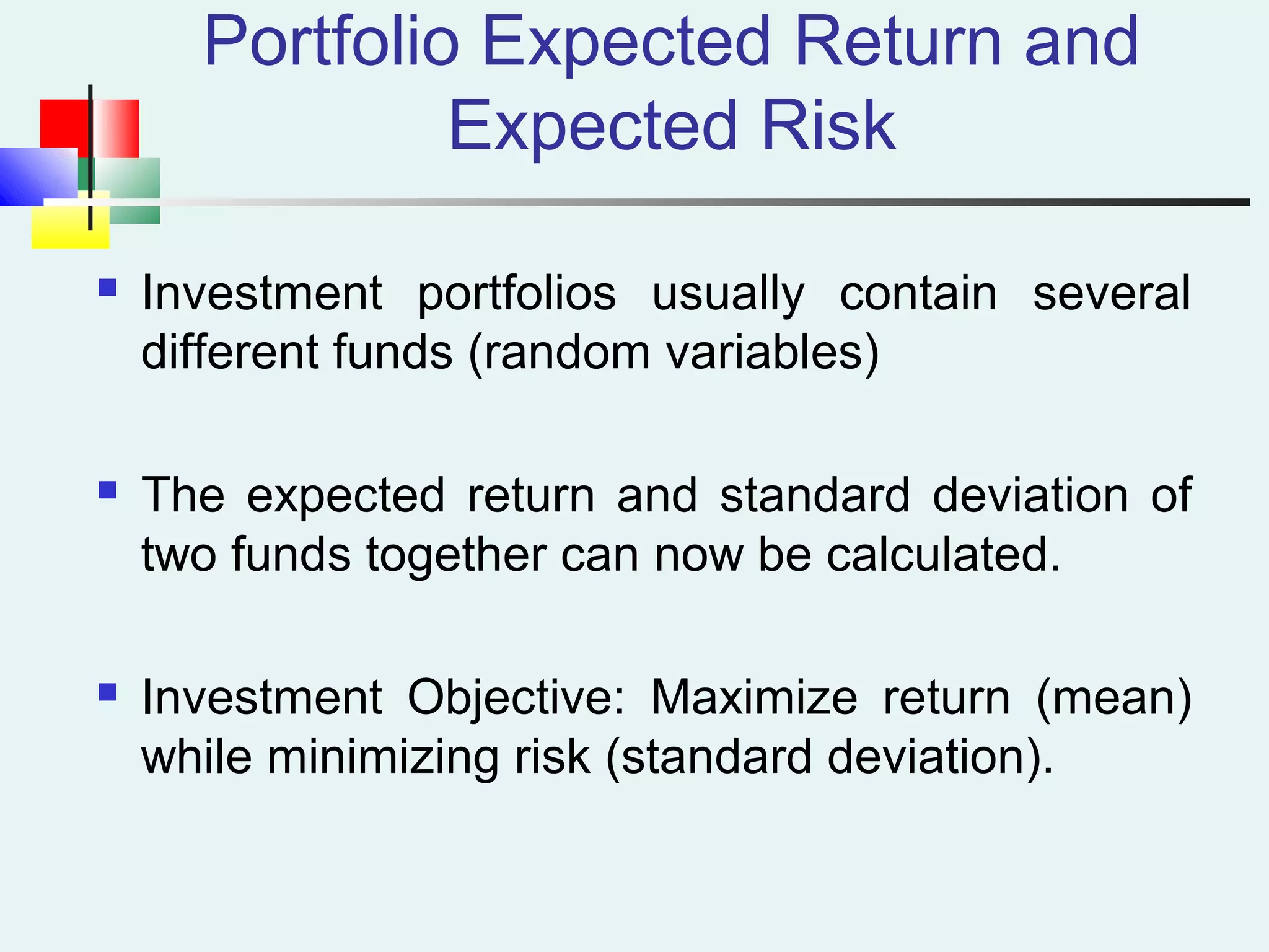
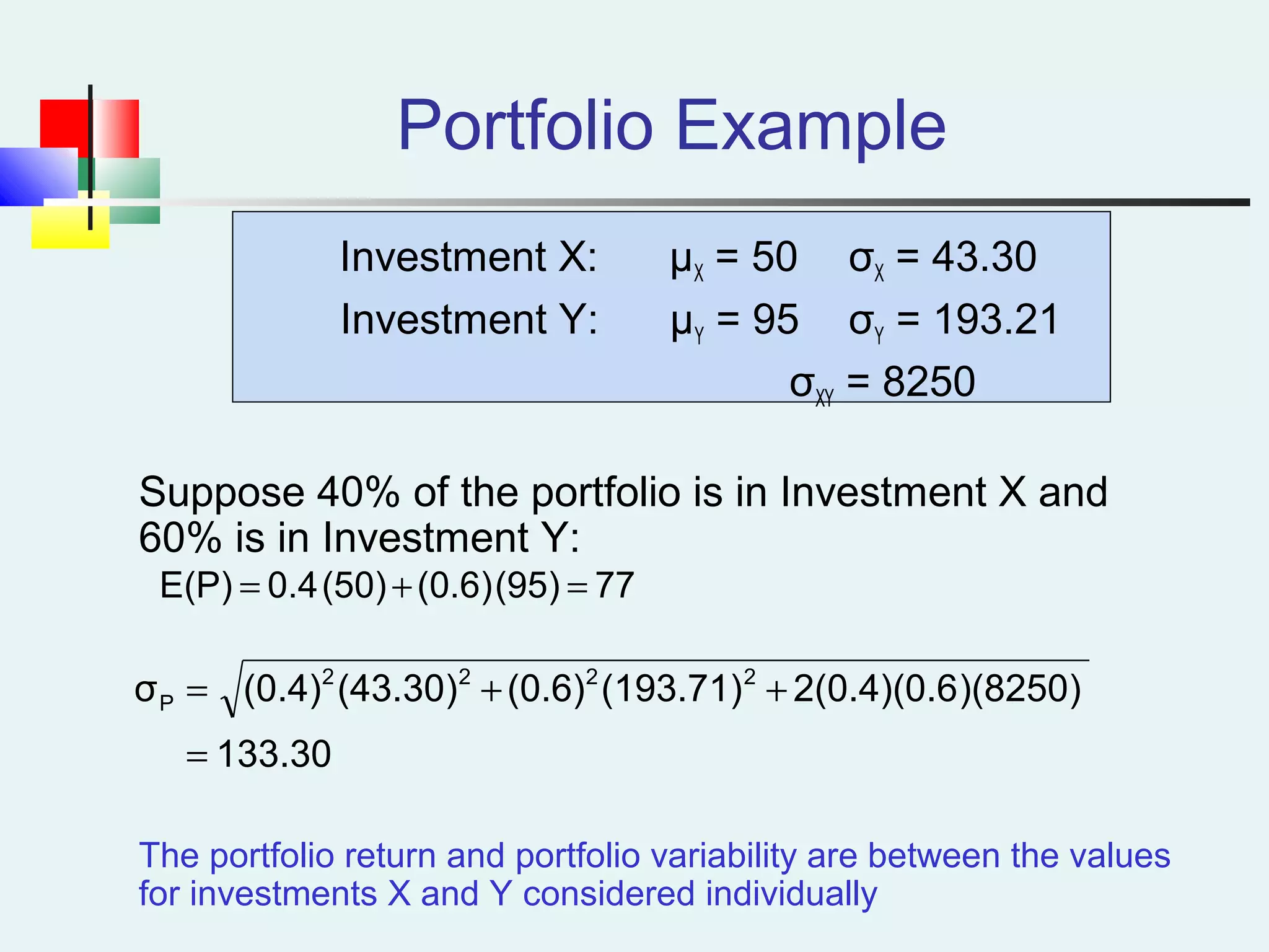
Analysis of investment returns illustrating expected values and standard deviations between funds.
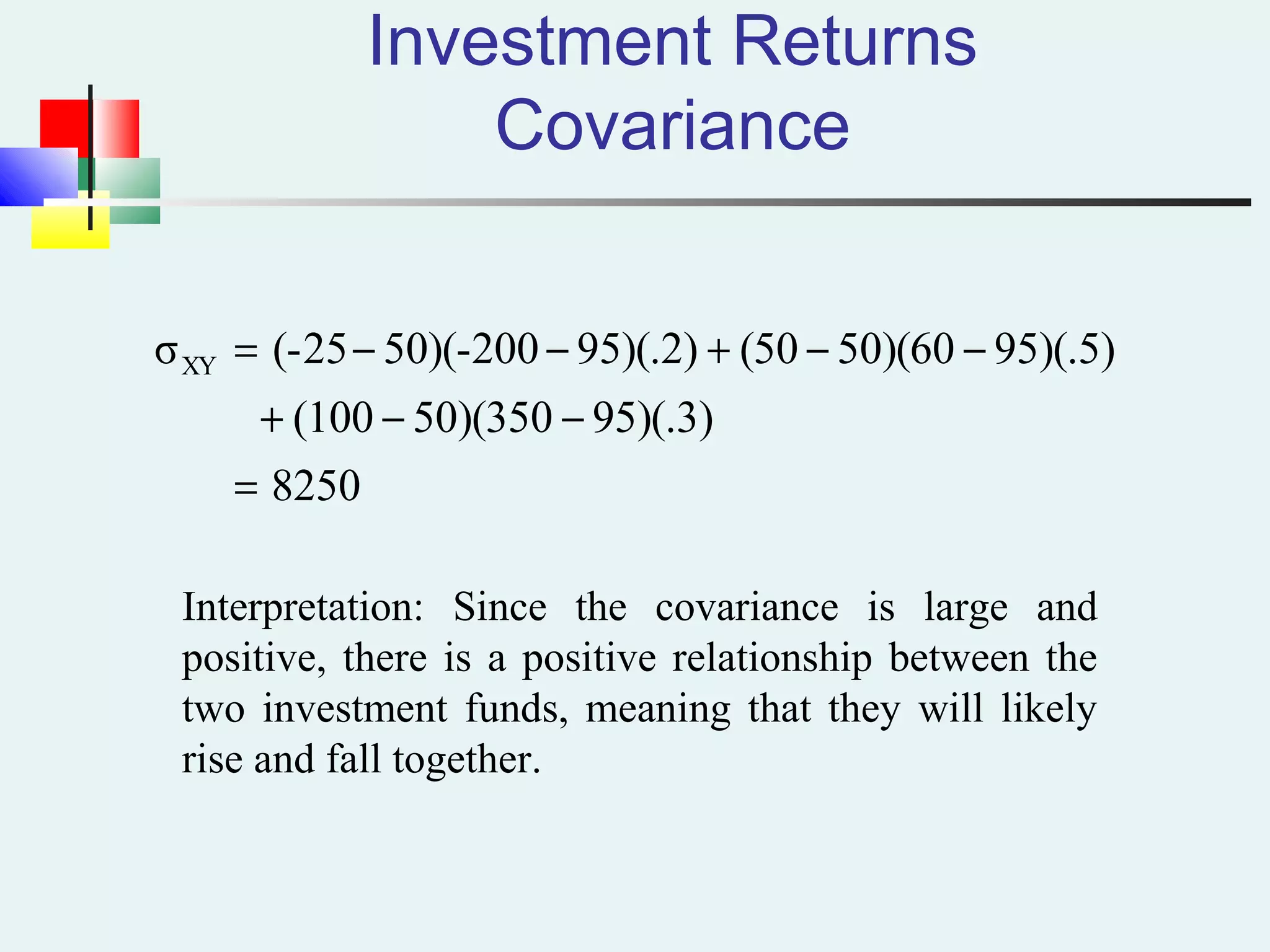
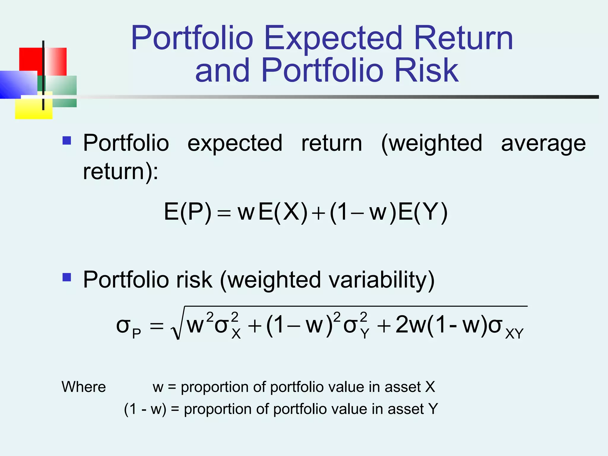
Describes covariance in the context of investments, detailing calculations for portfolio returns and risks.
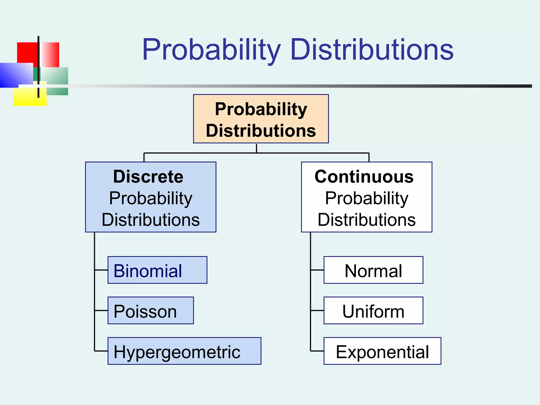
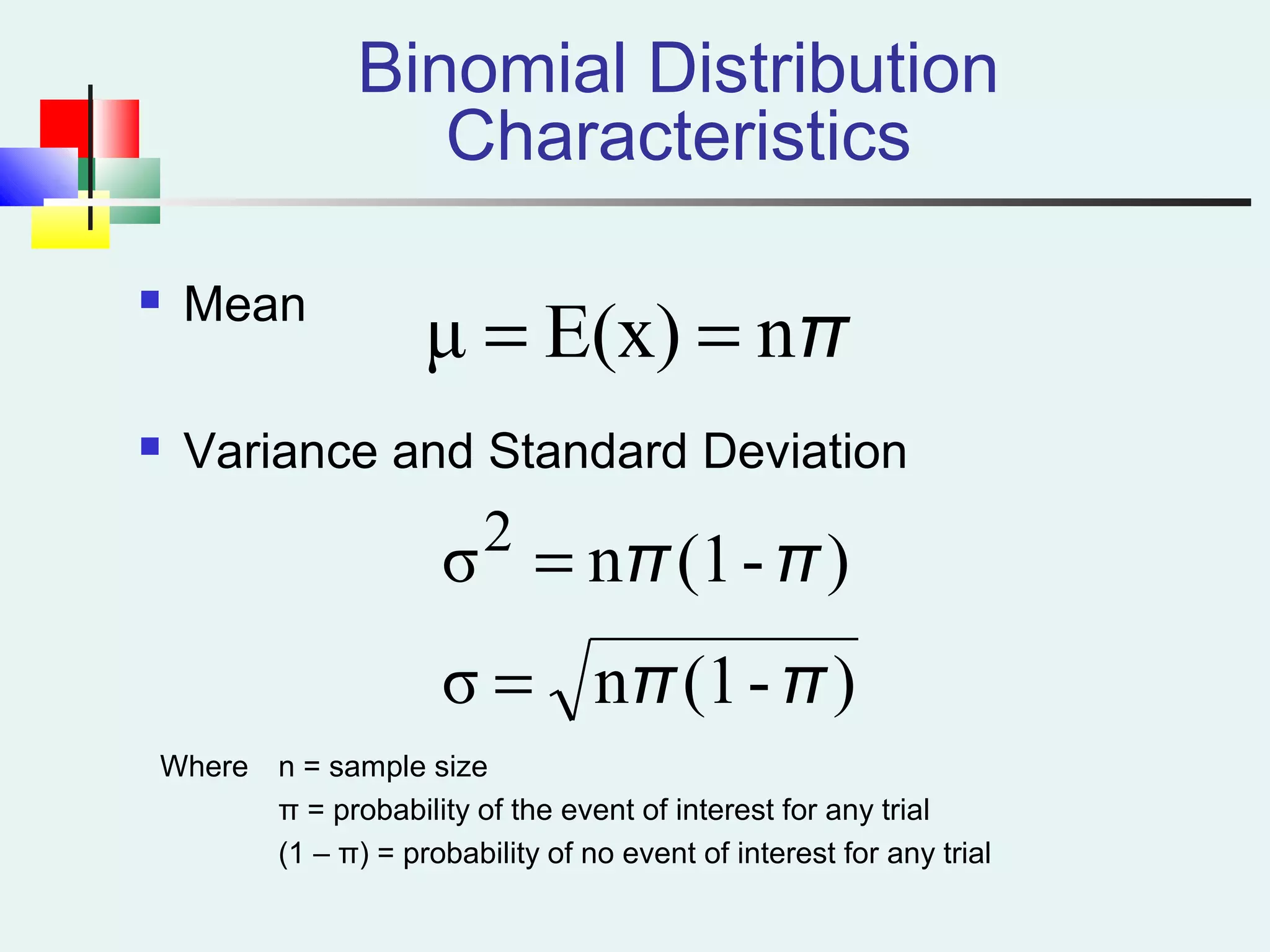
Overview of continuous and discrete probability distributions including binomial and Poisson distributions.
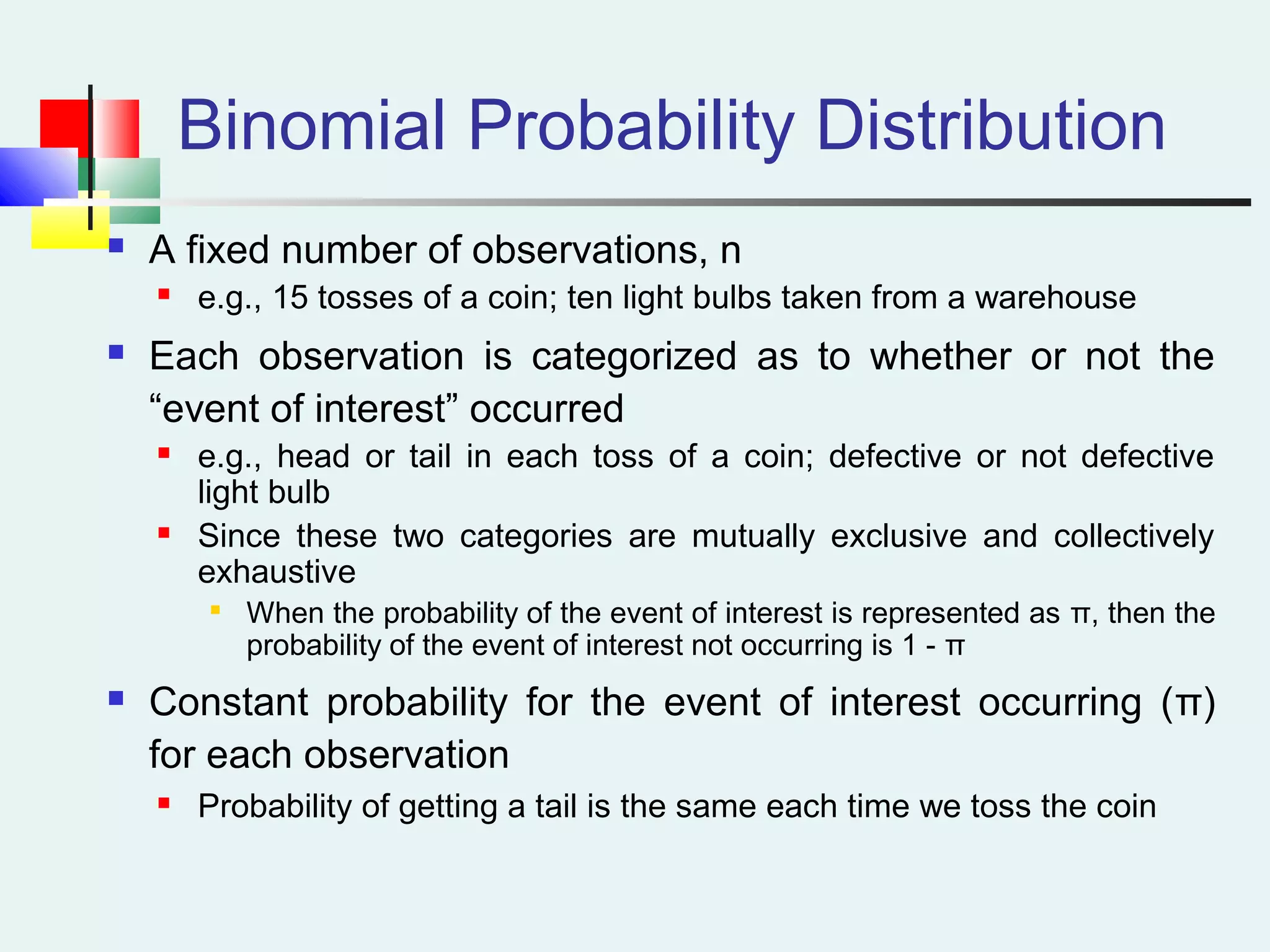
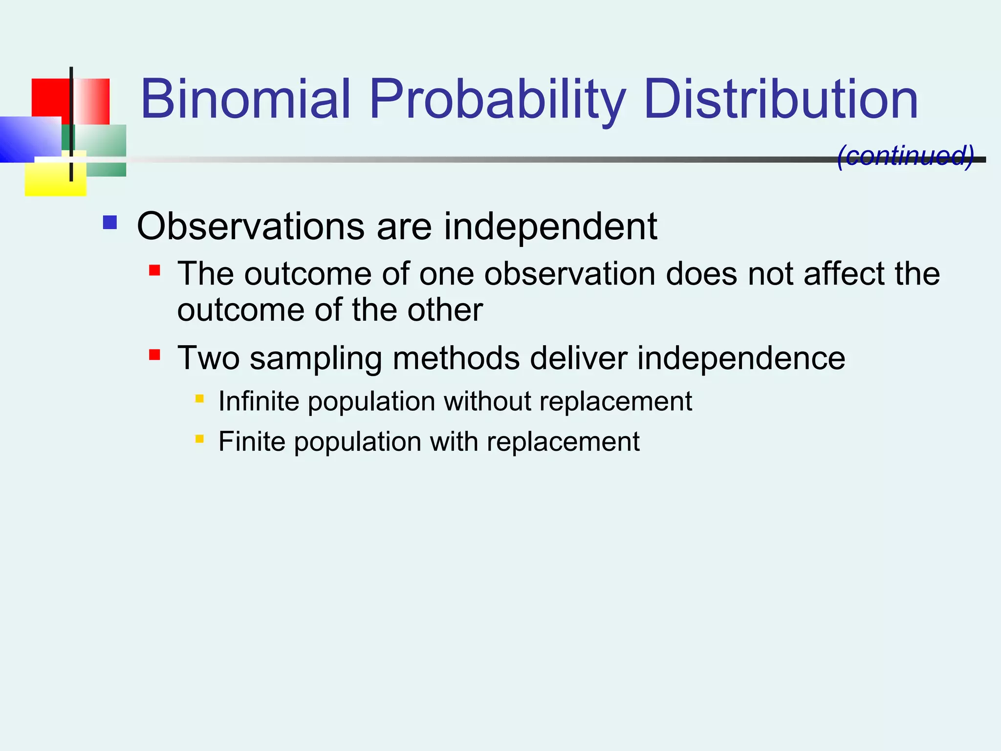
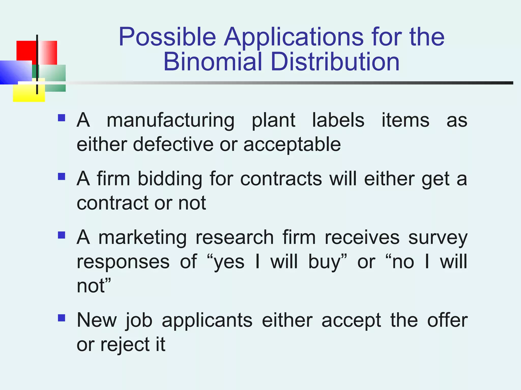
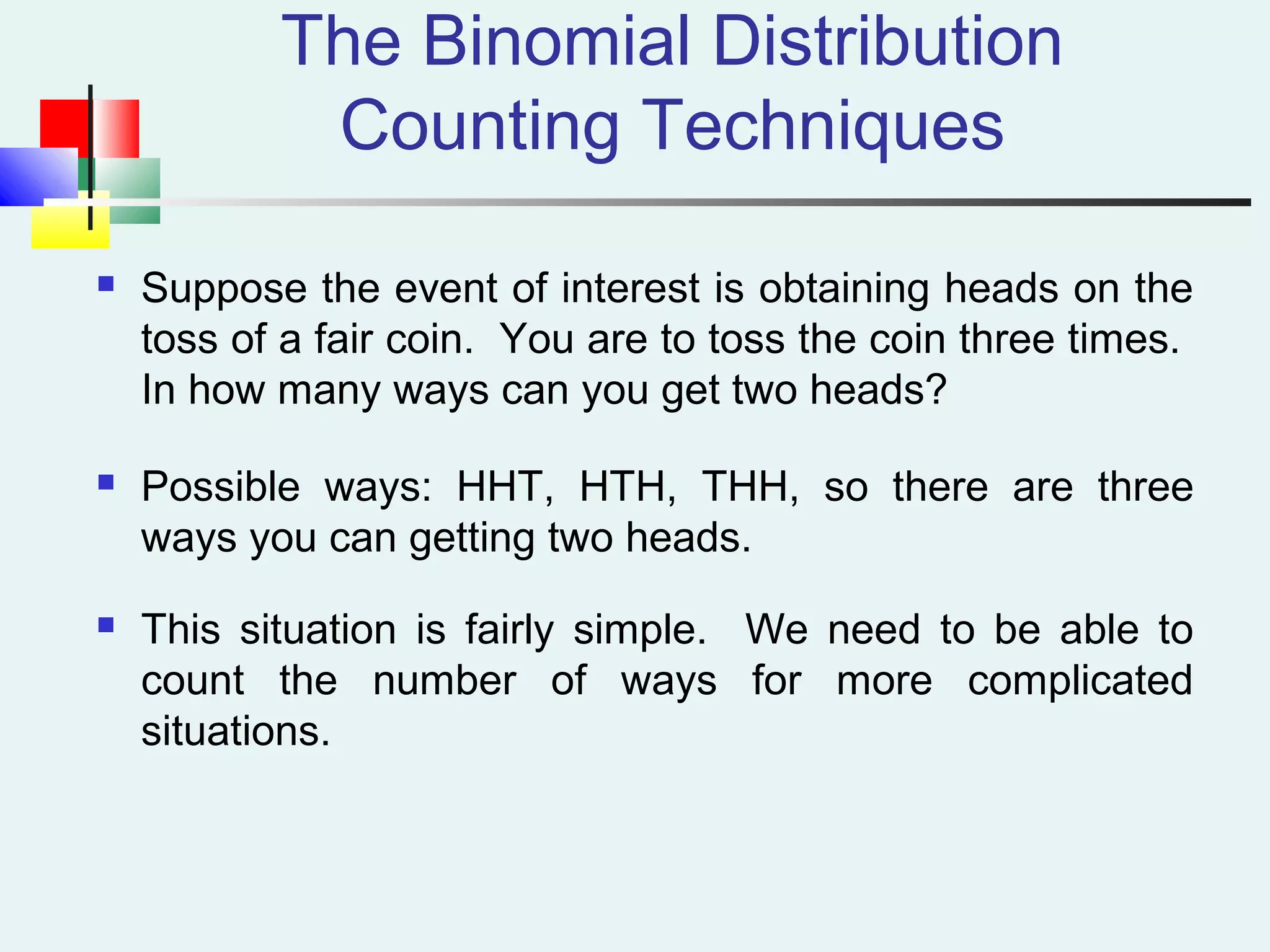
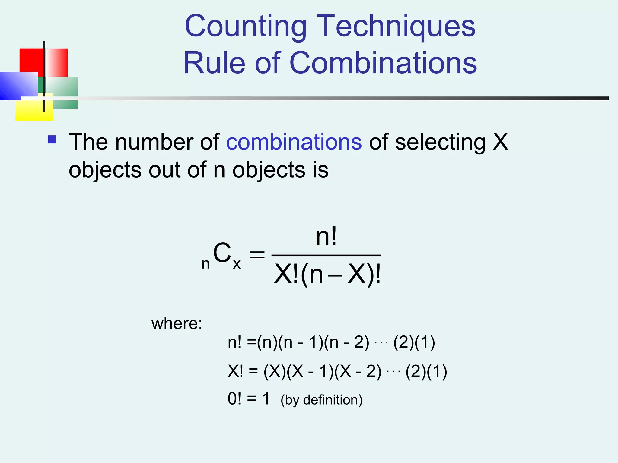
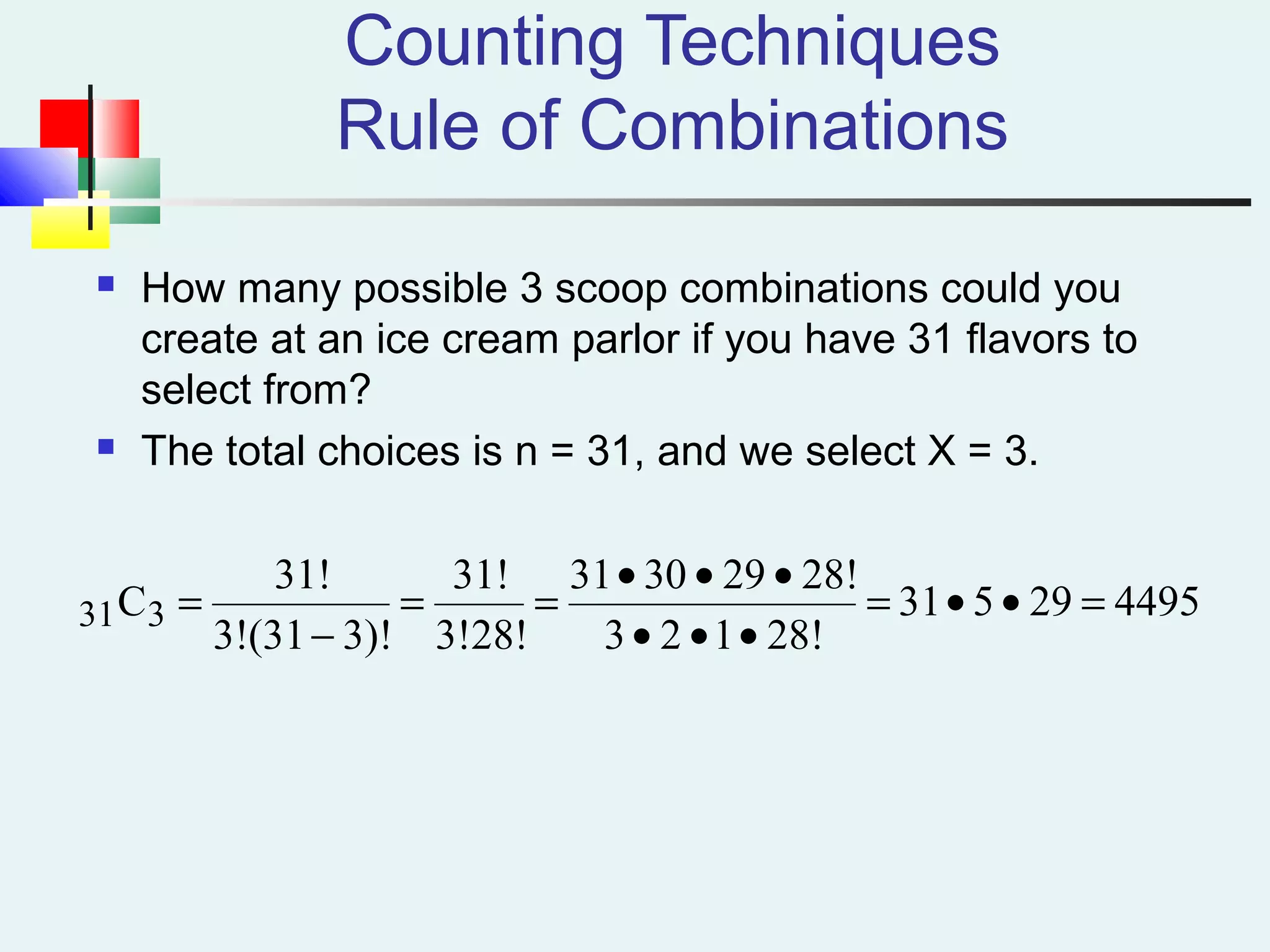
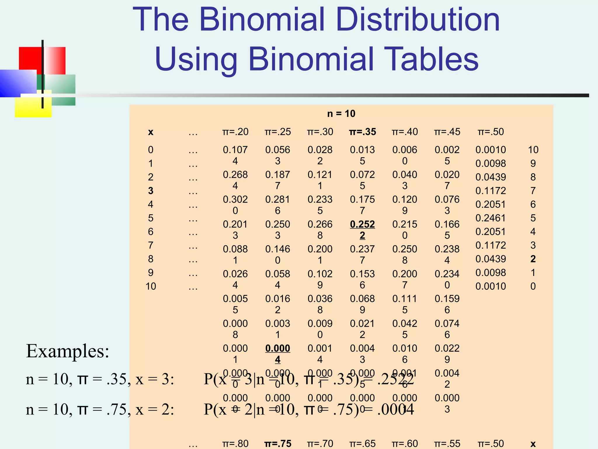
Details on properties of binomial distributions and counting techniques for outcomes.
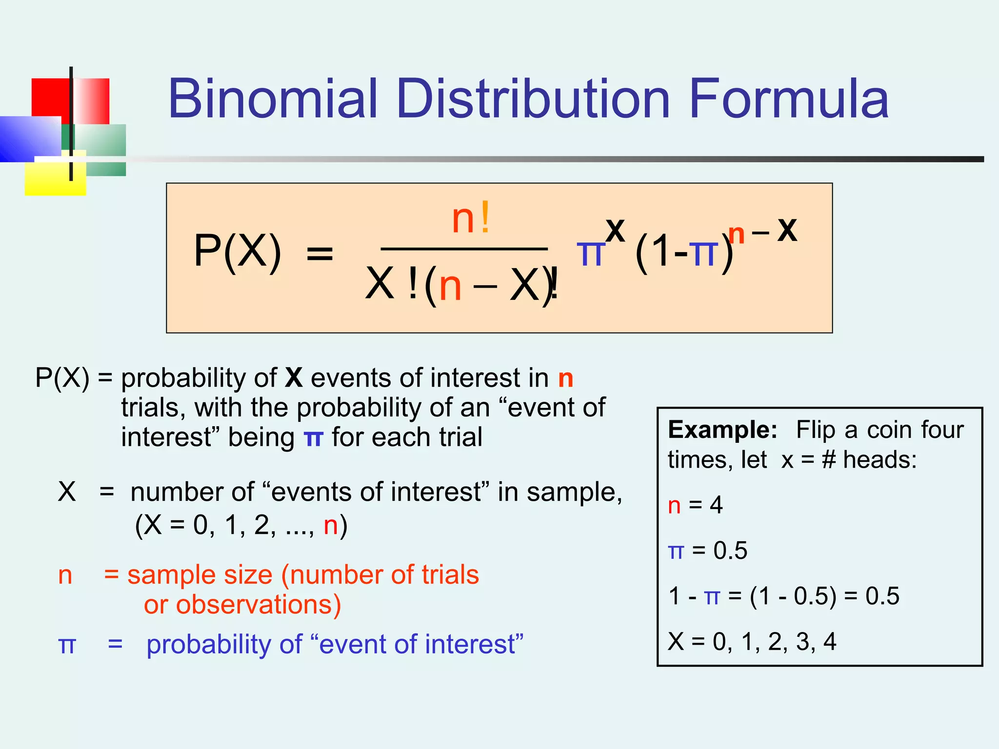
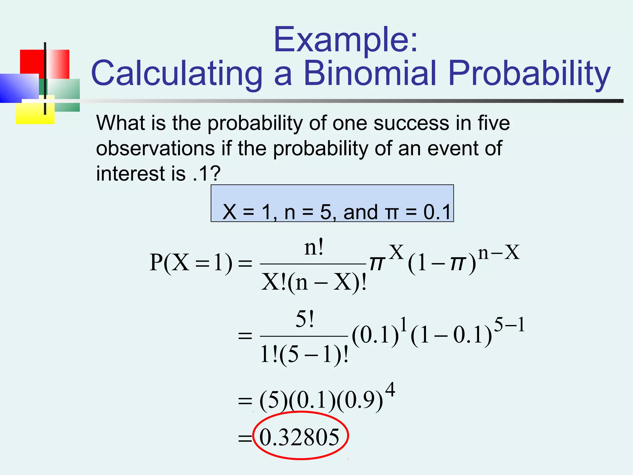
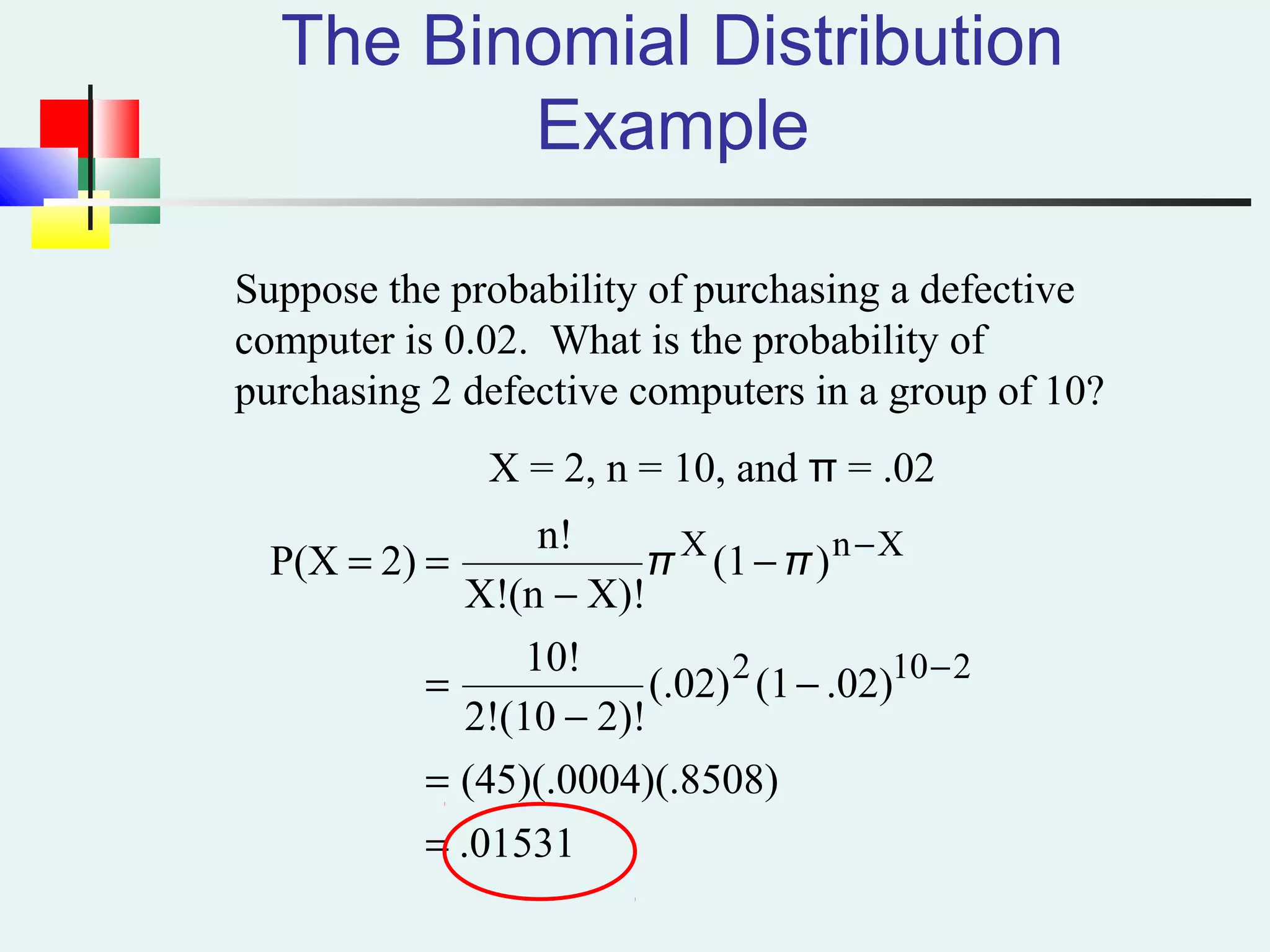
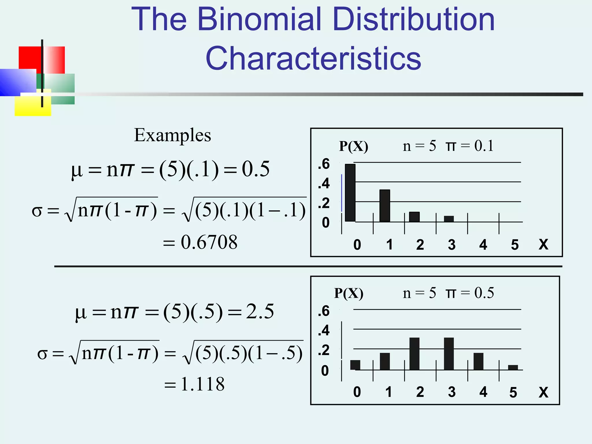
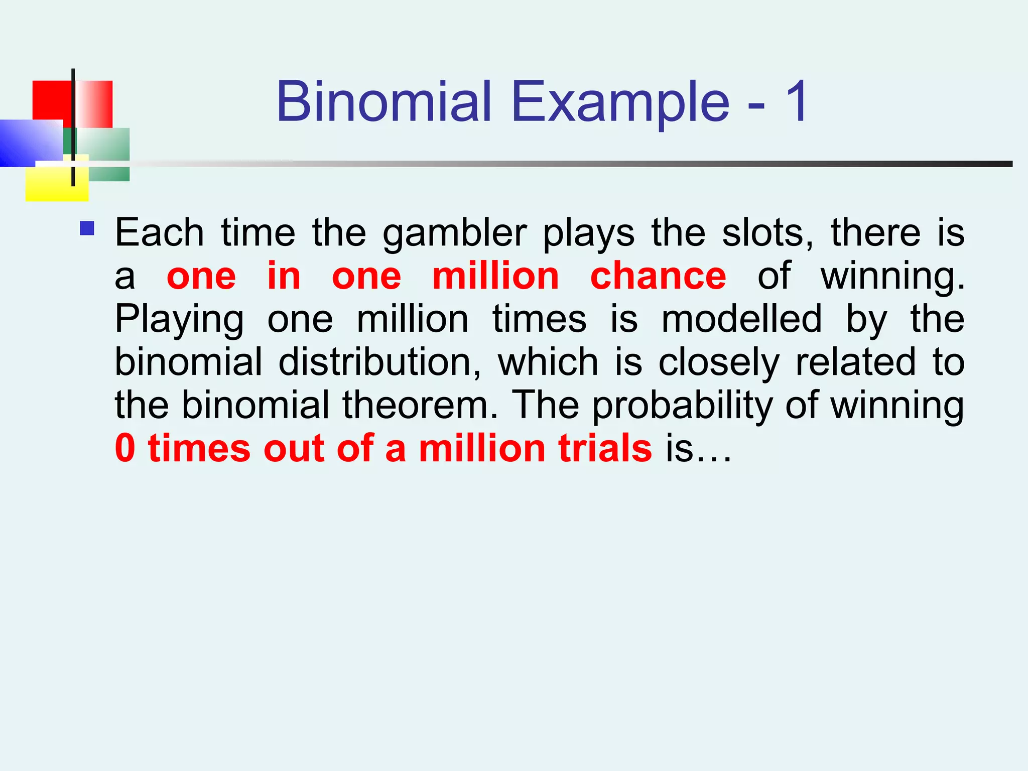
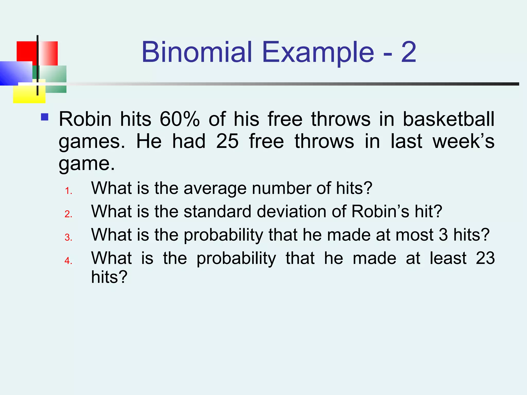
Calculating probabilities and expected values using the binomial distribution formula.
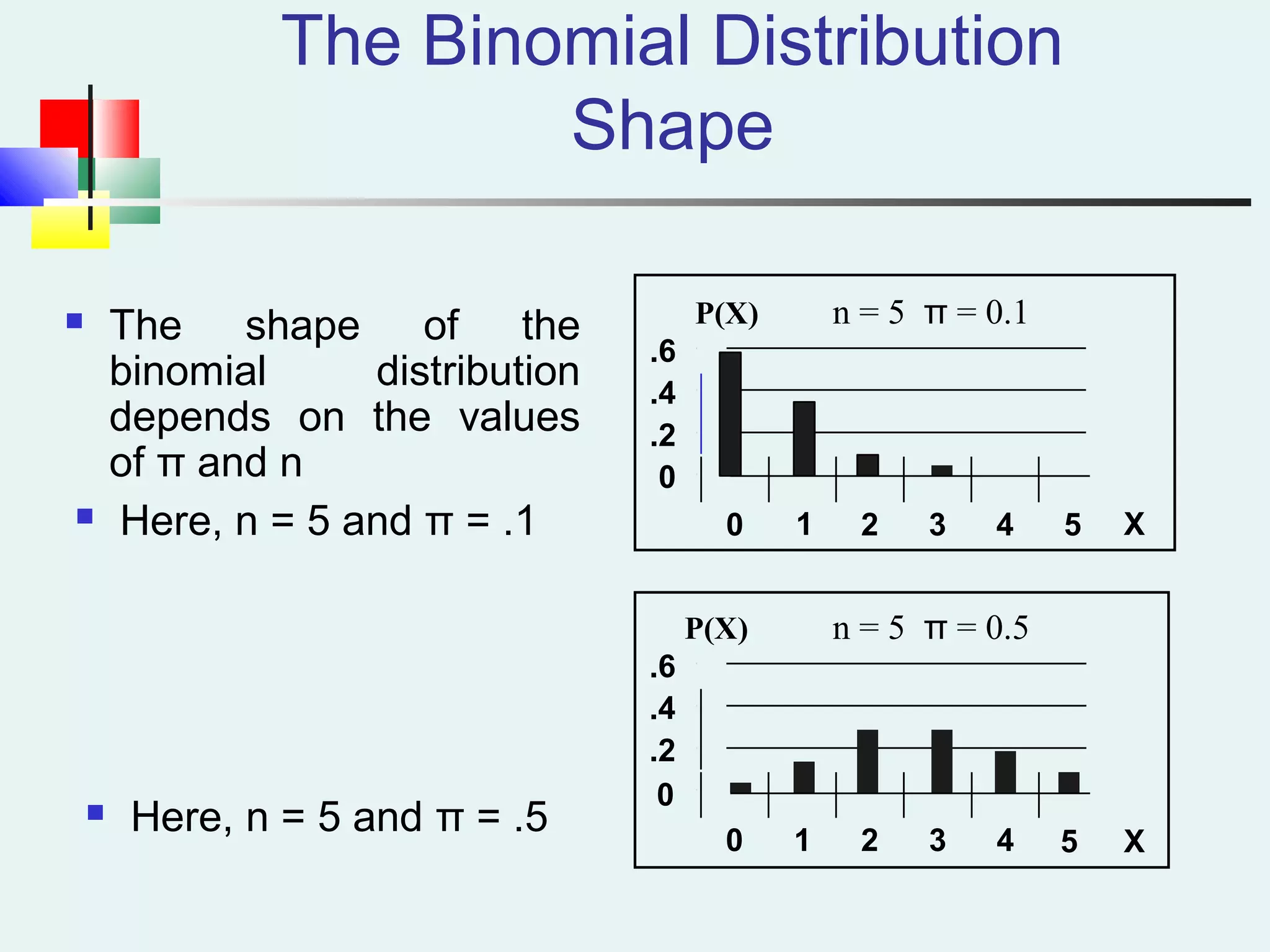
Analysis of the shape and characteristics of the binomial distribution across examples.
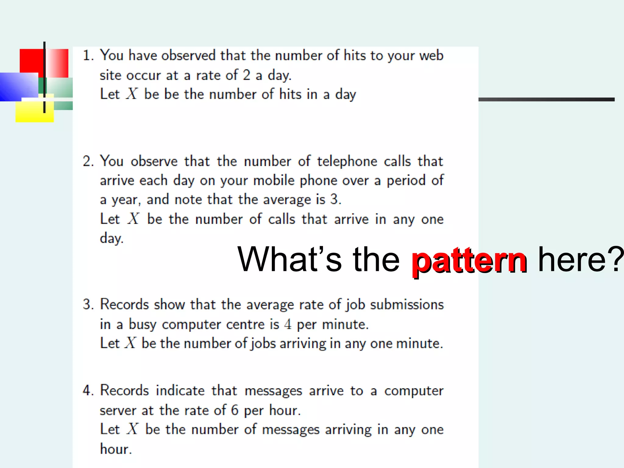
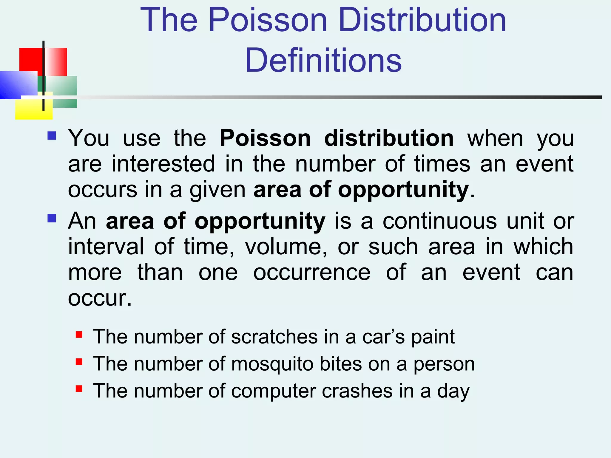
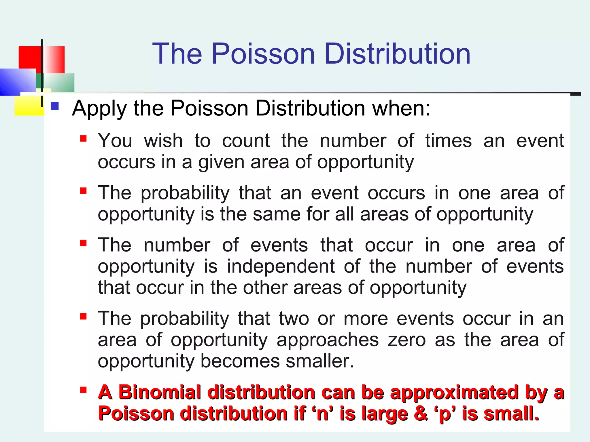
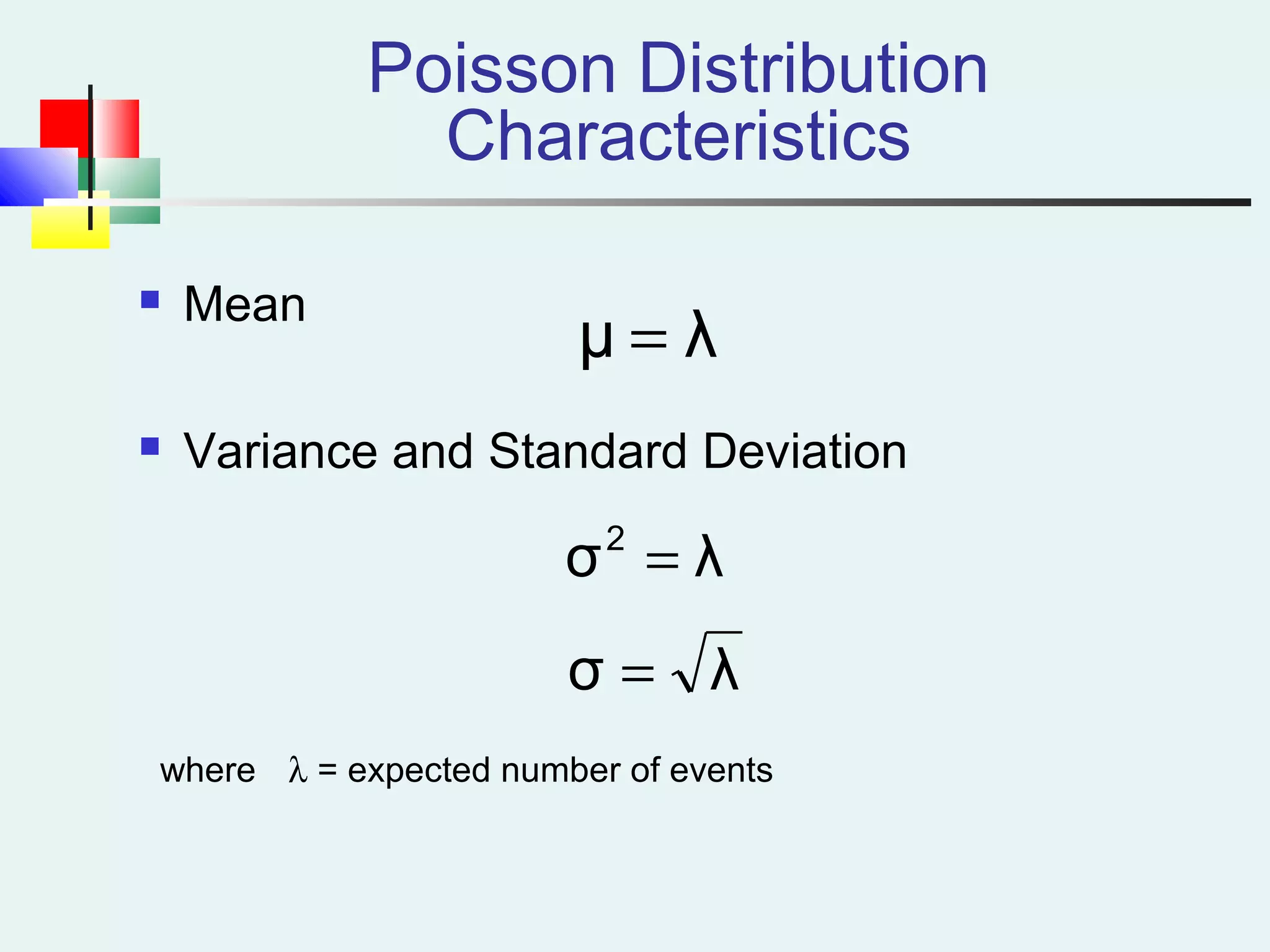
Definitions and characteristics of Poisson distribution for occurrences in a set interval.
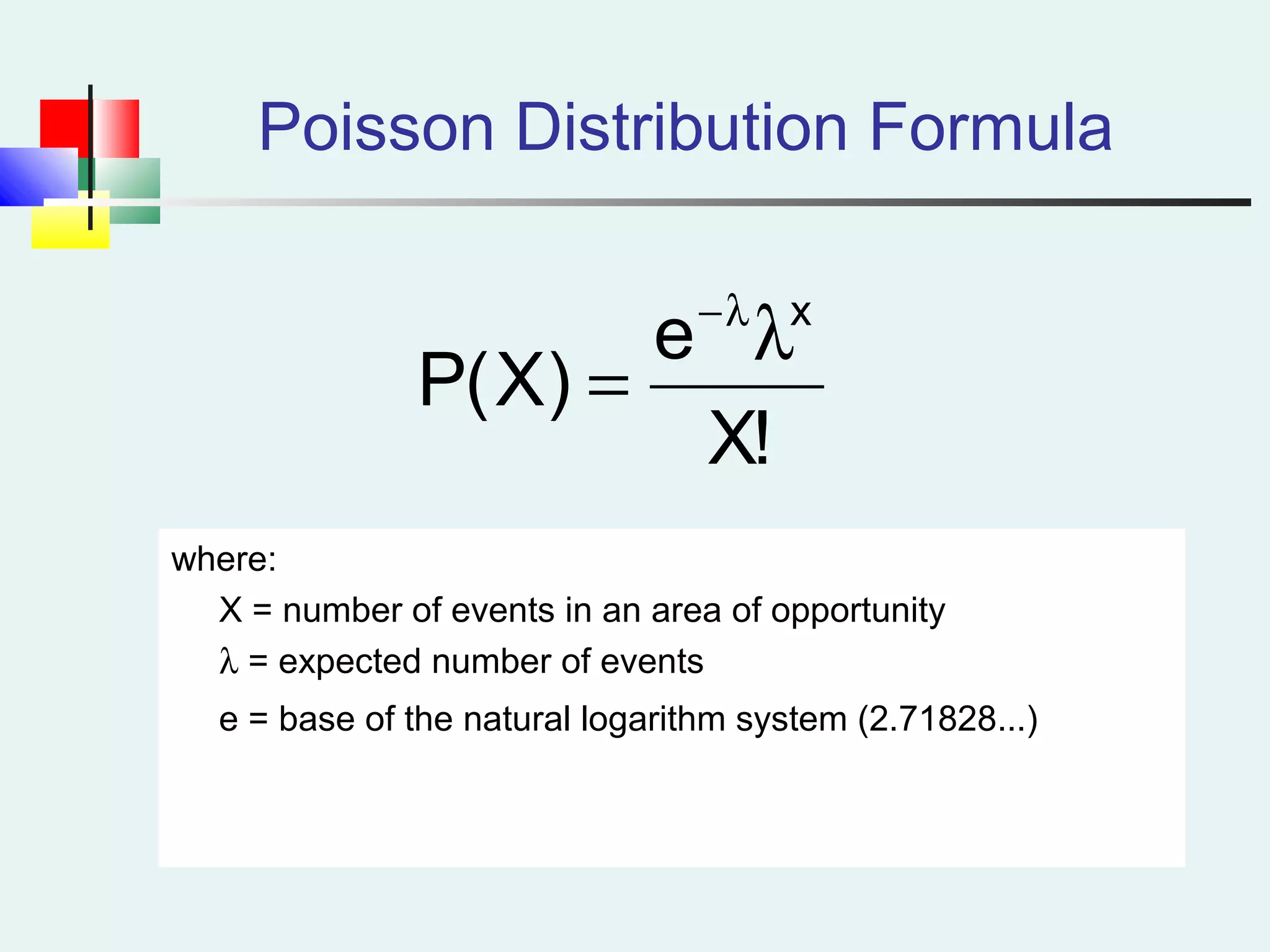
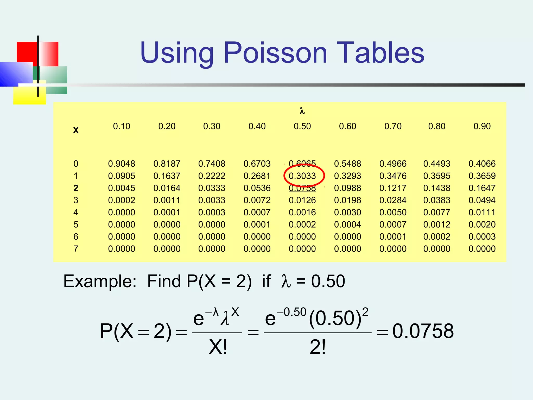
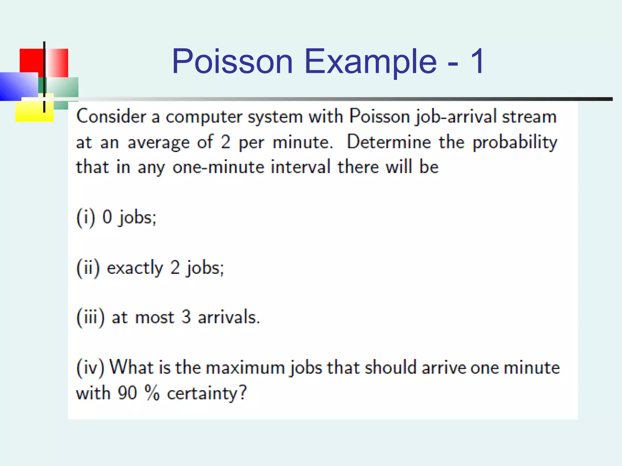
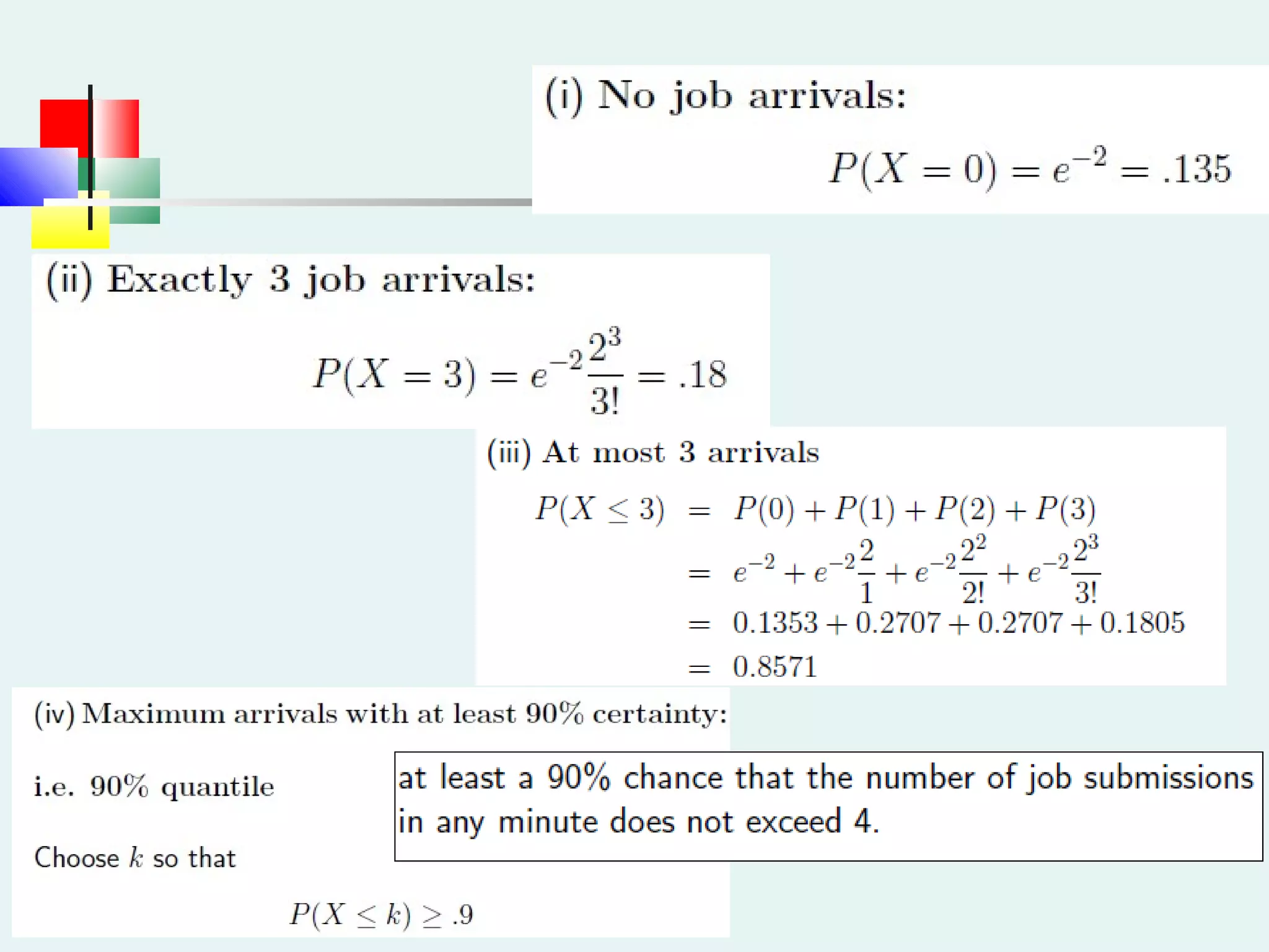
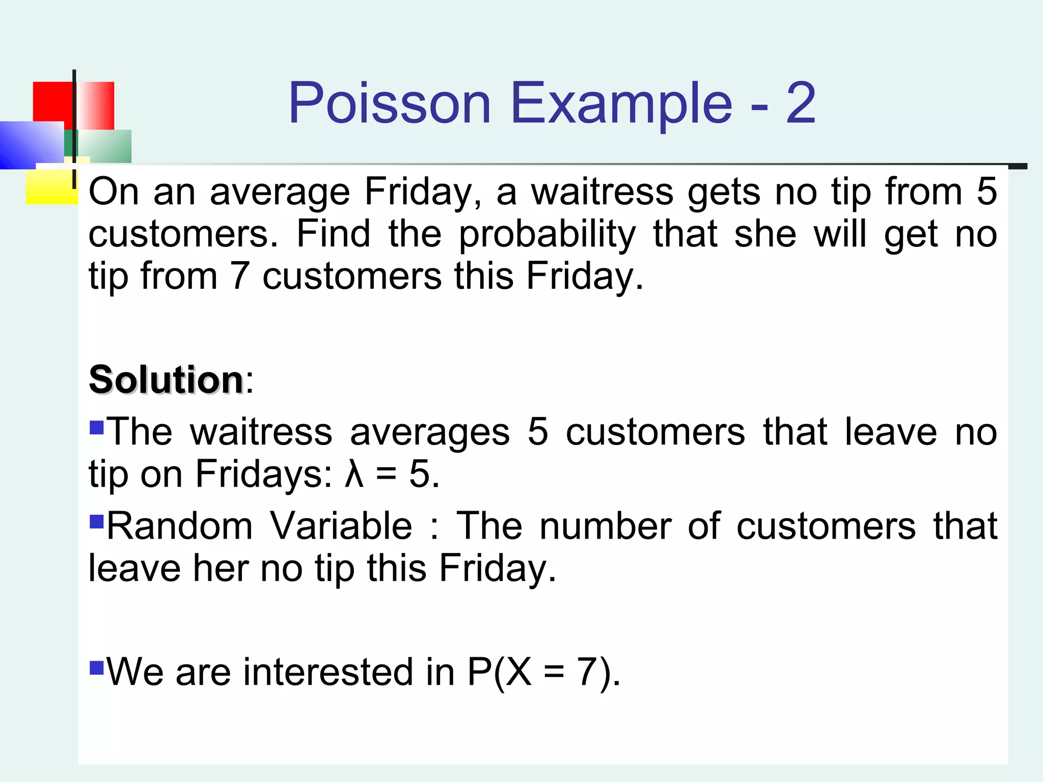
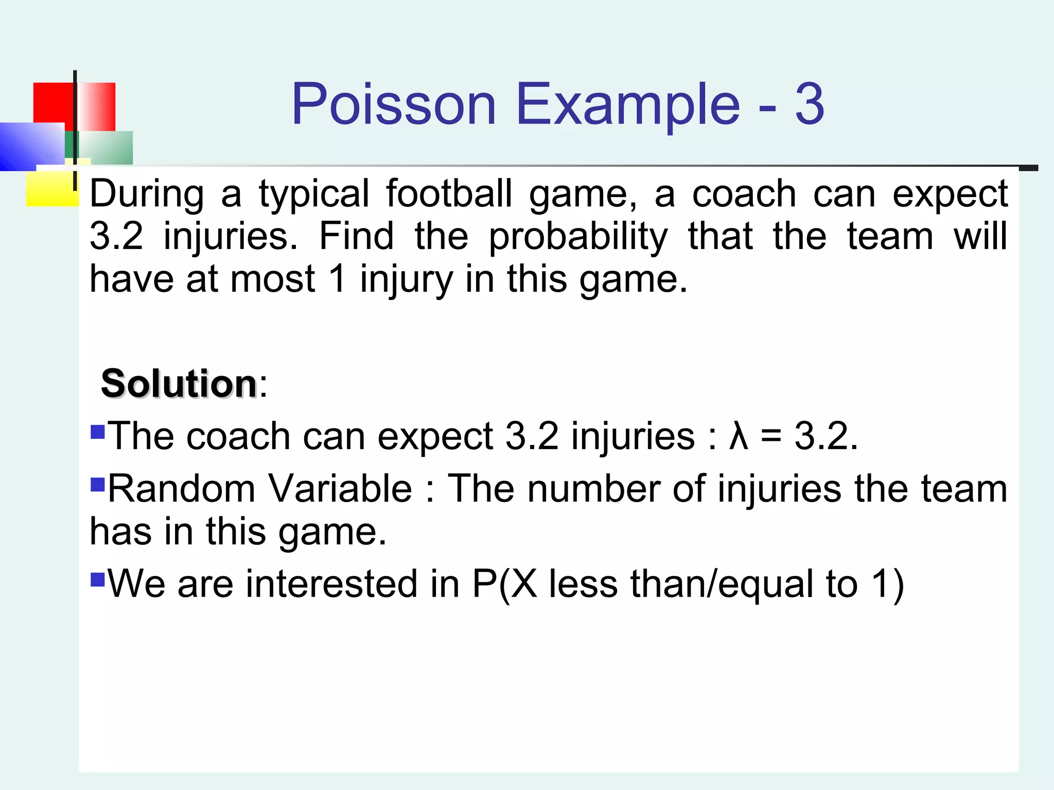
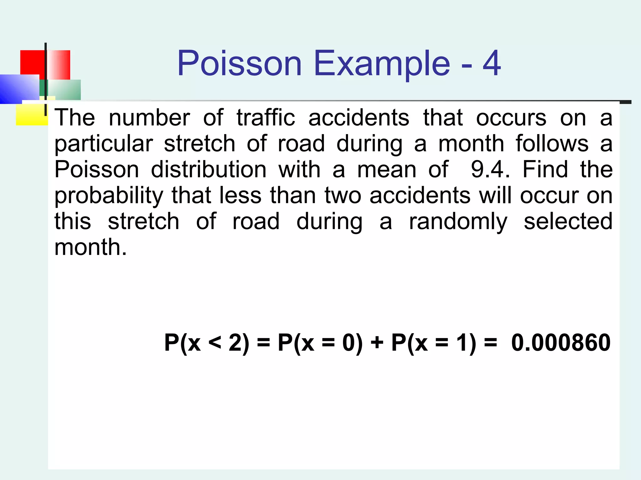
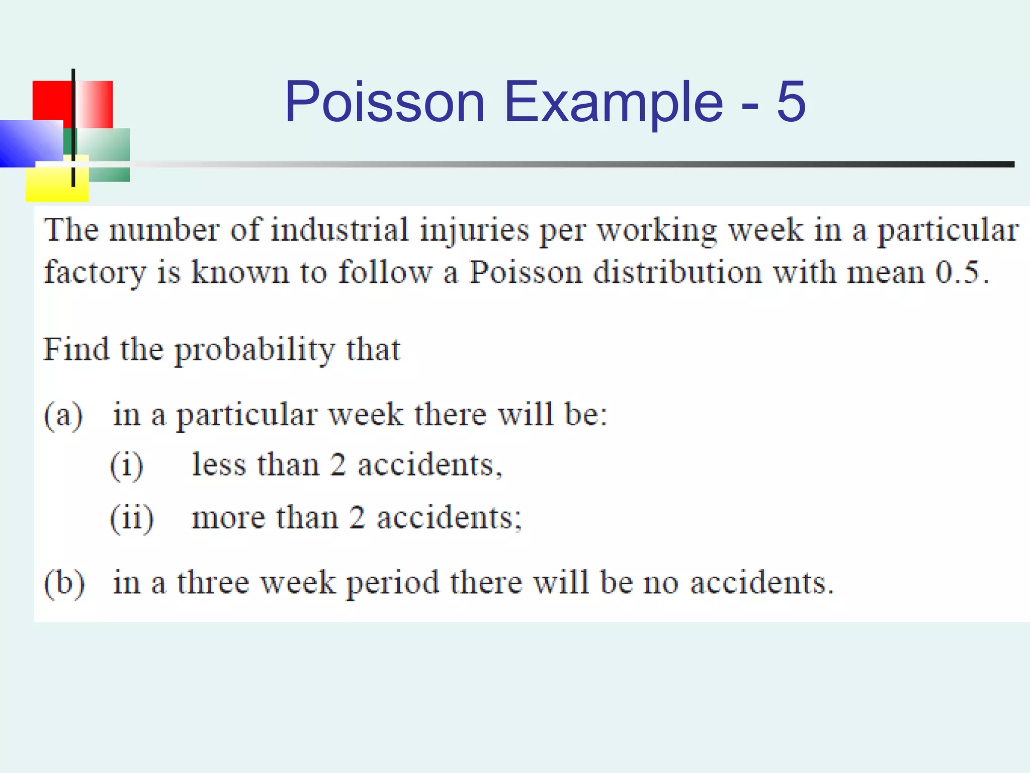
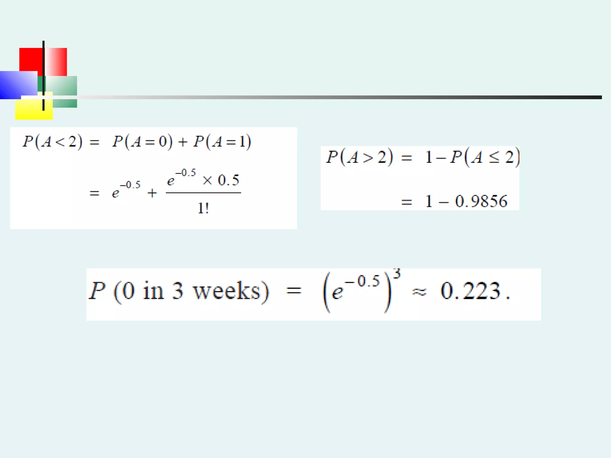
Practical examples calculating probabilities with the Poisson distribution for various scenarios.
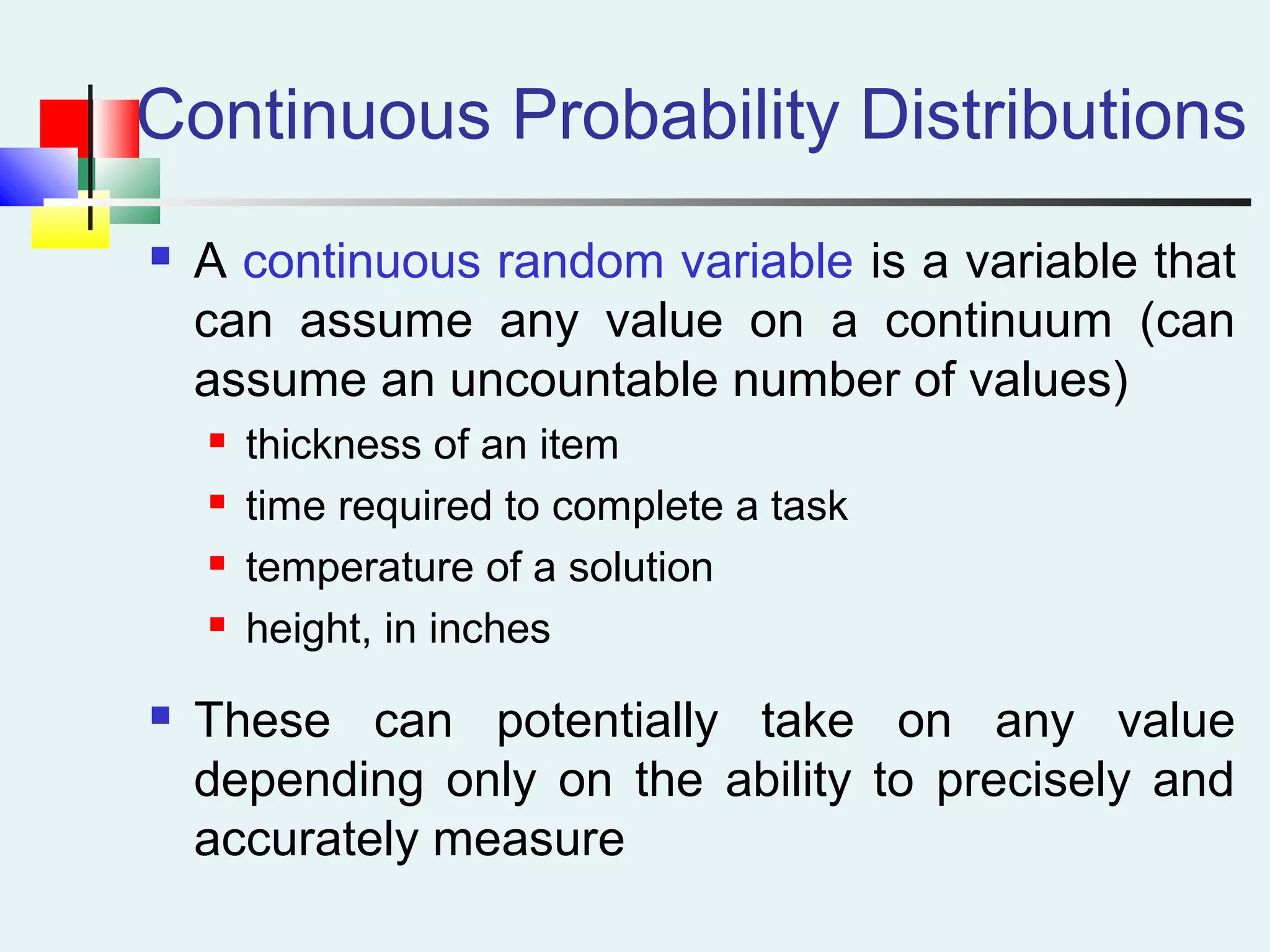
Introduction to continuous probability distributions, defining variables that can take any value.
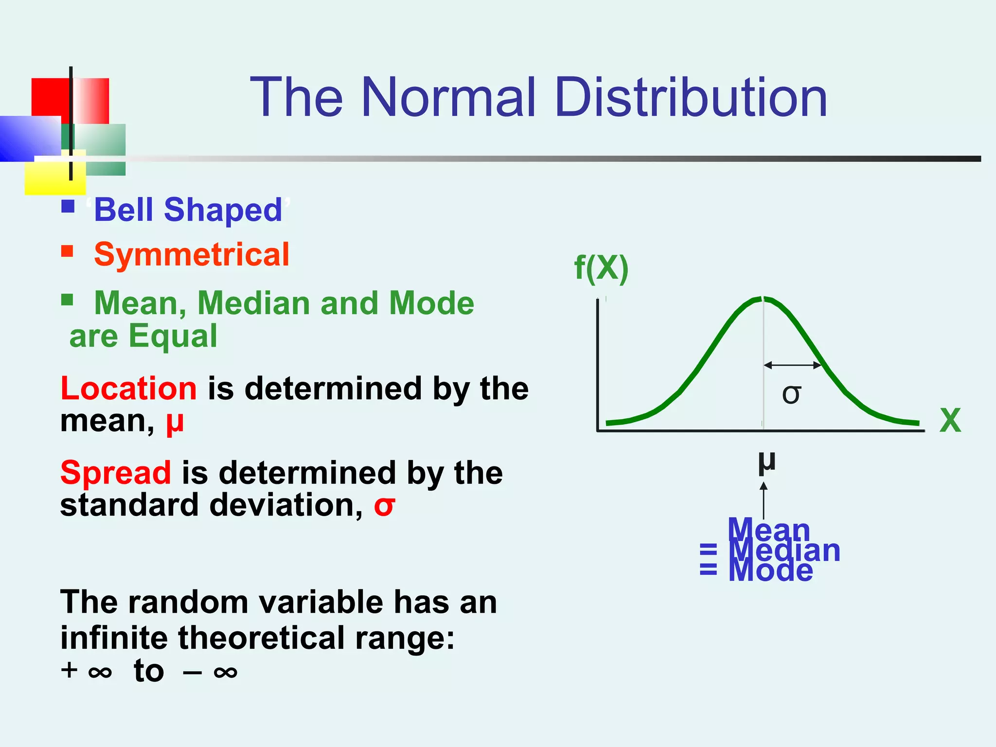
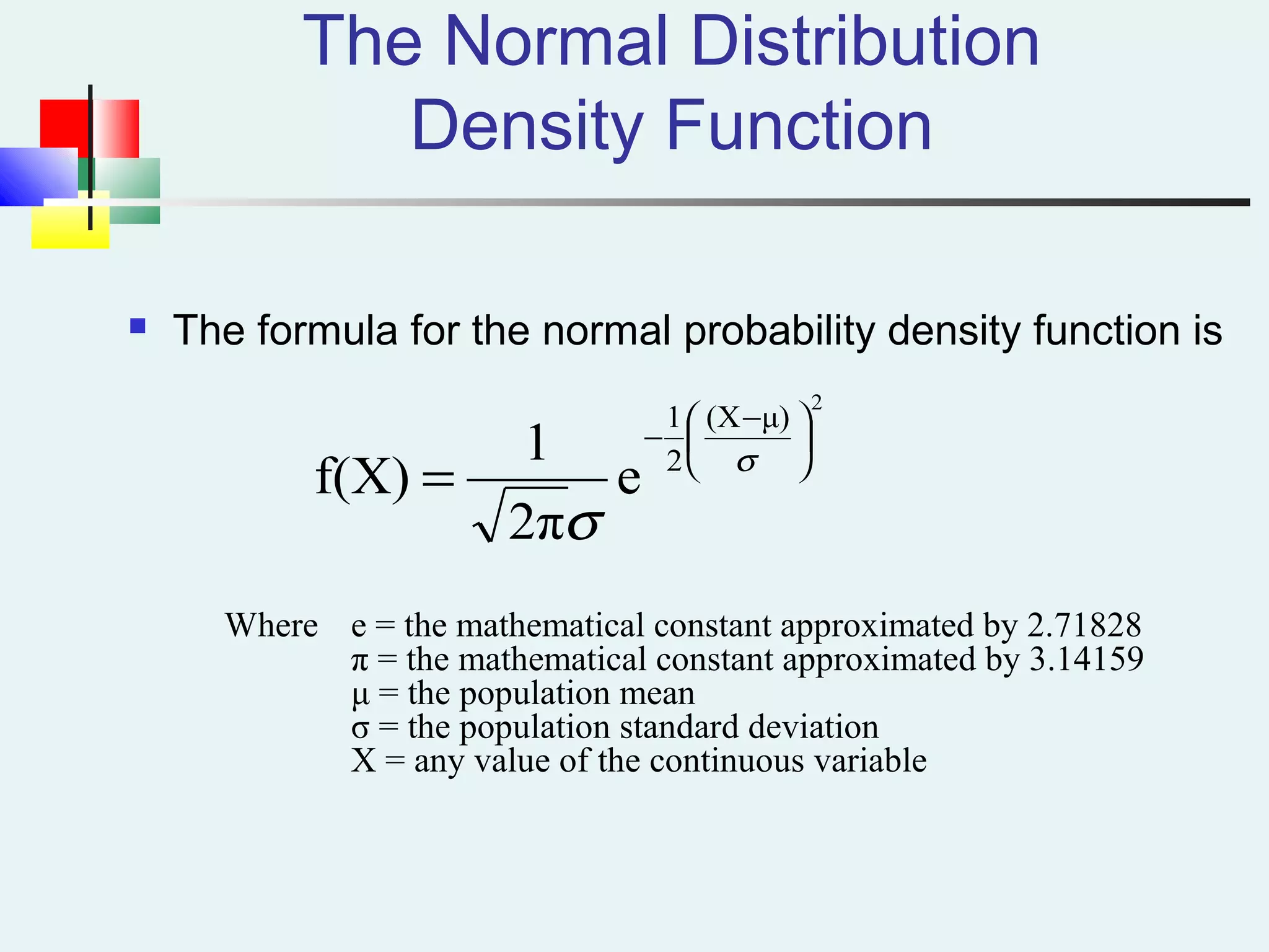
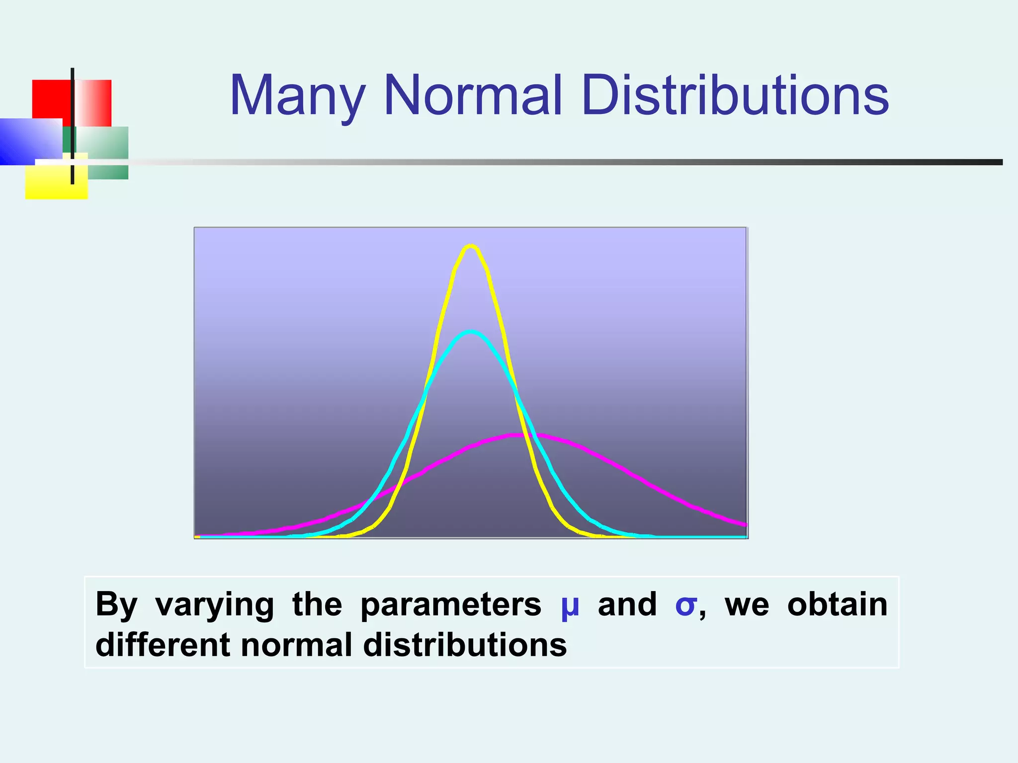
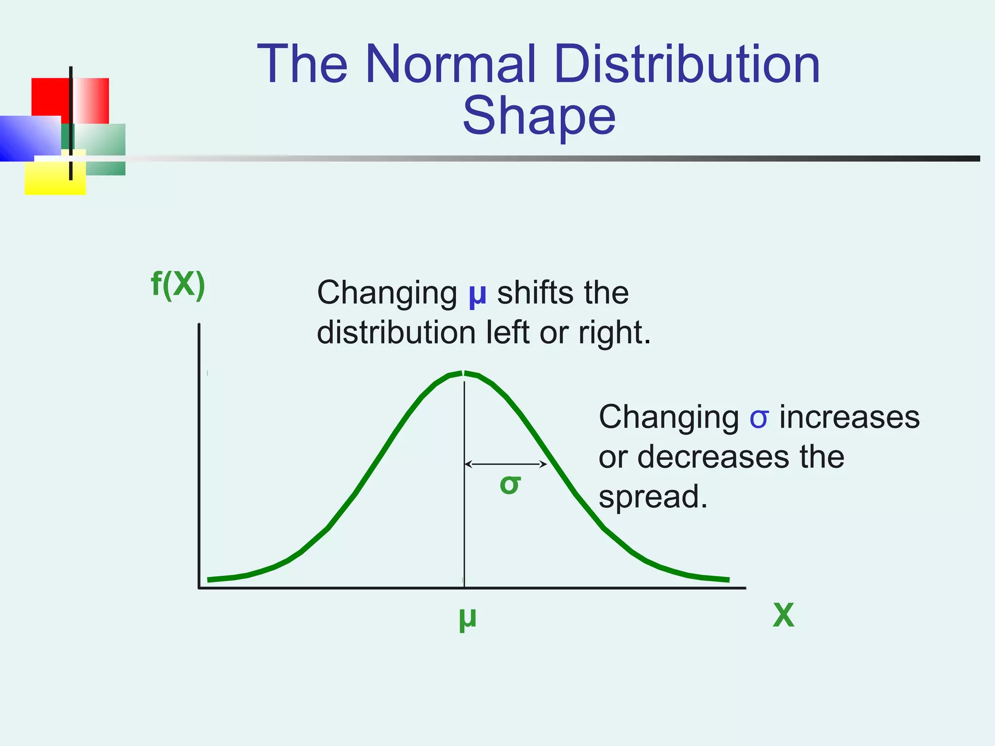
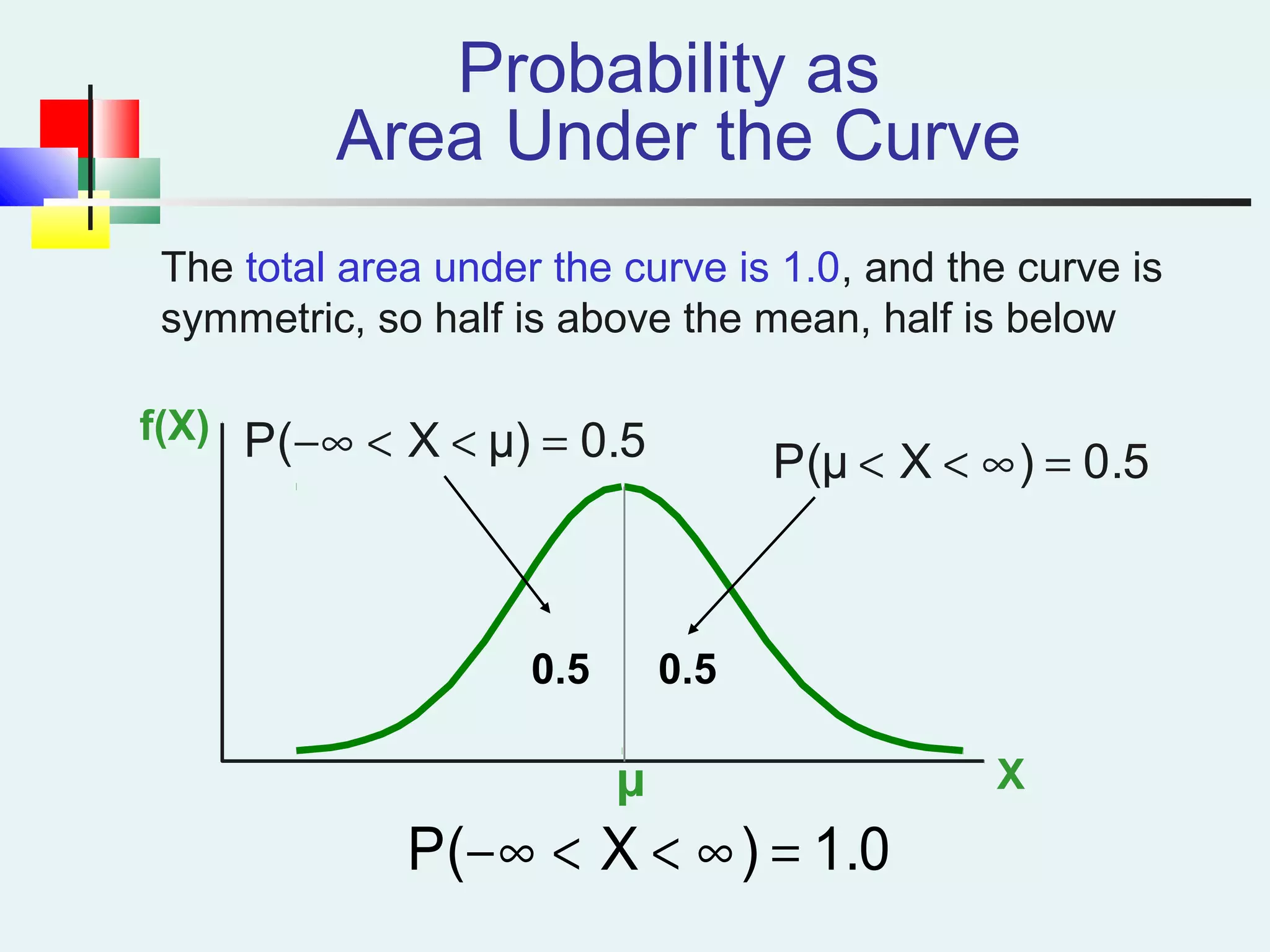
Characteristics of normal distribution, including definition, symmetry, and properties.
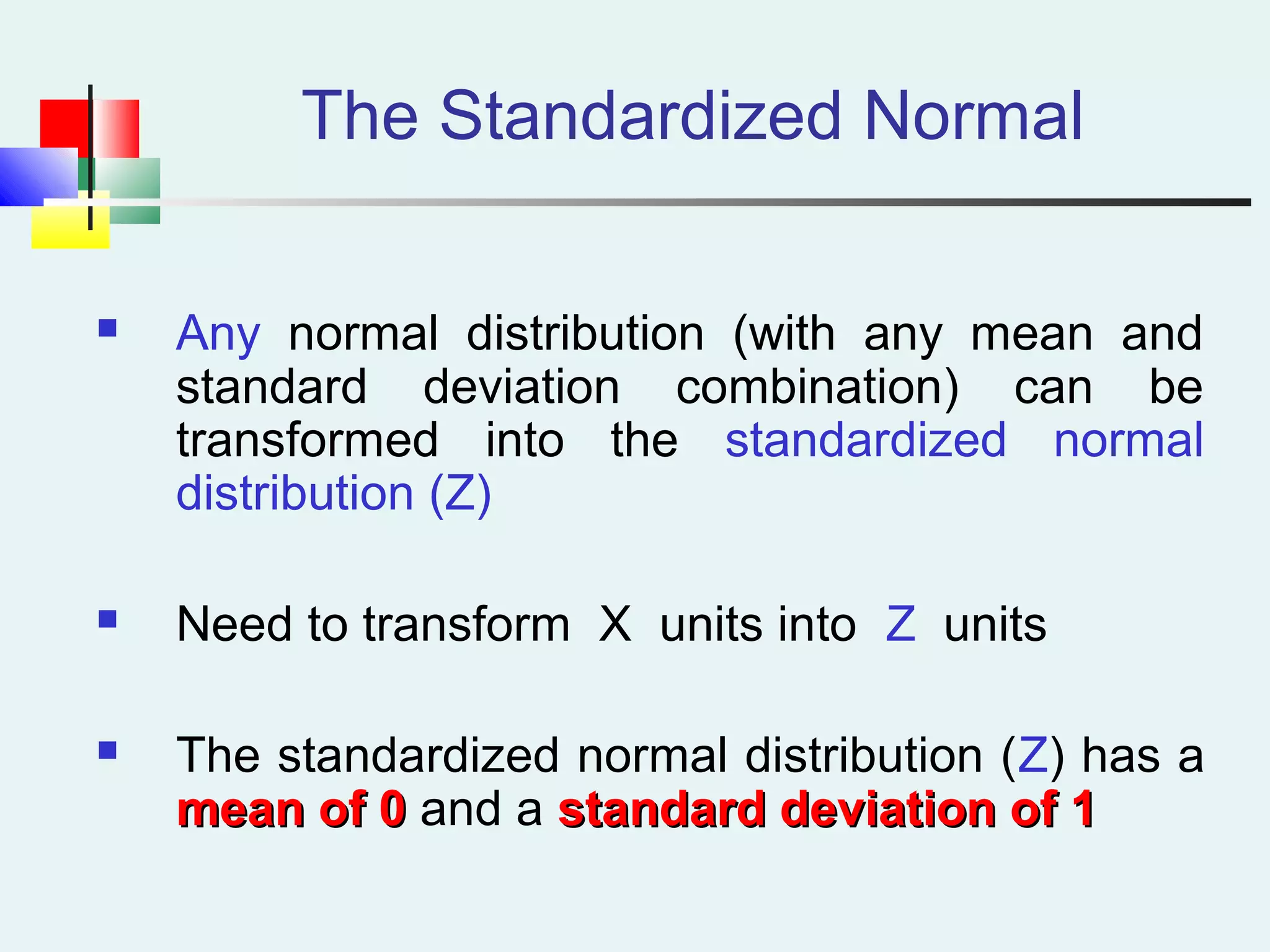
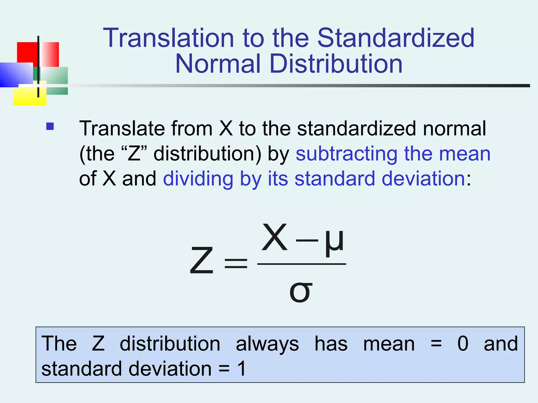
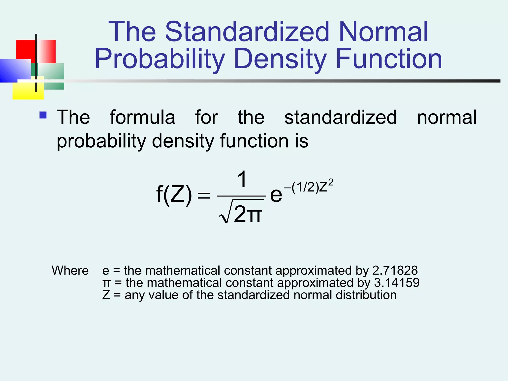
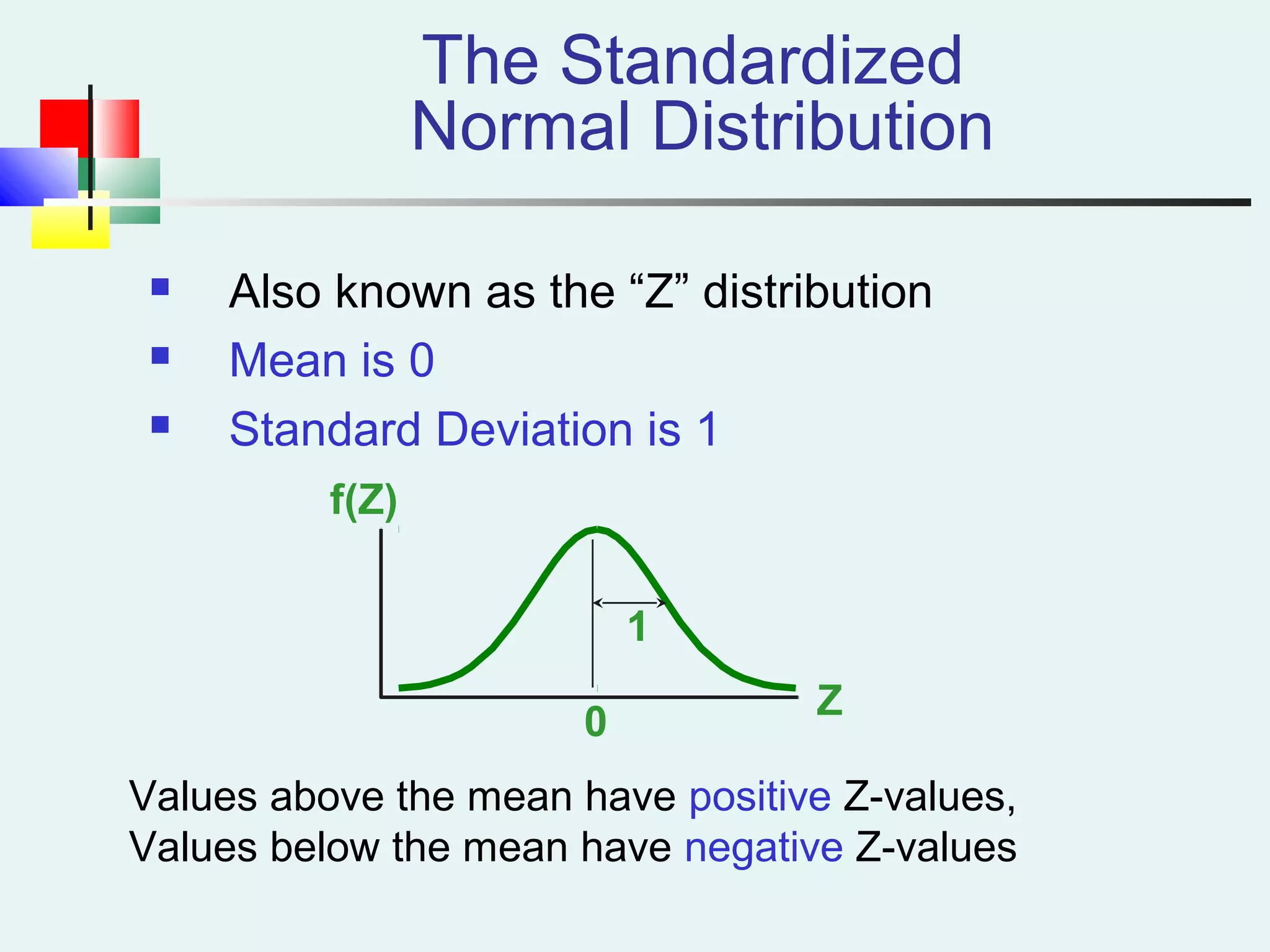
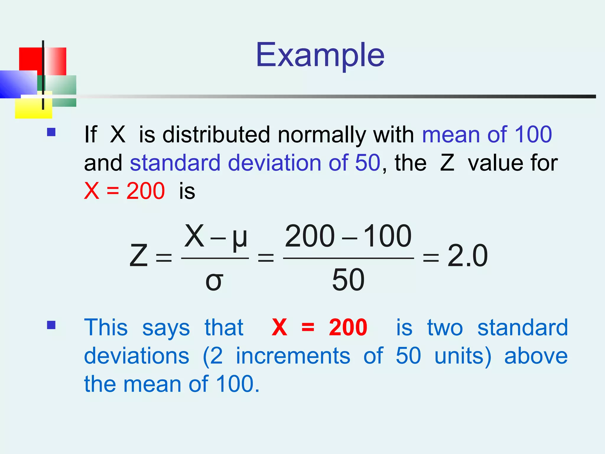
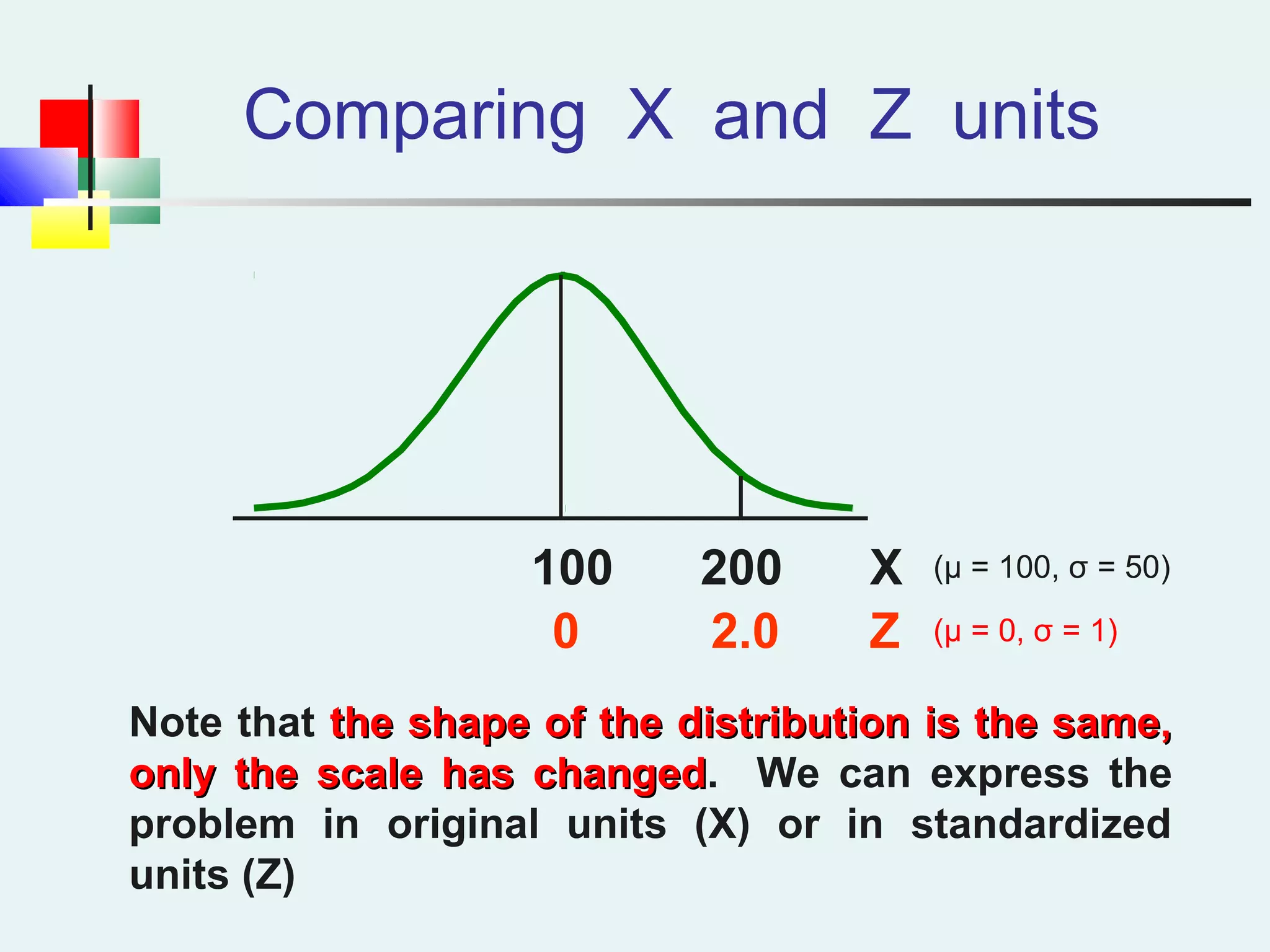
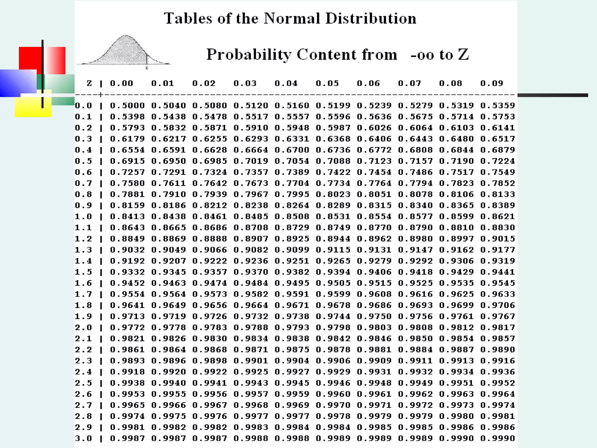
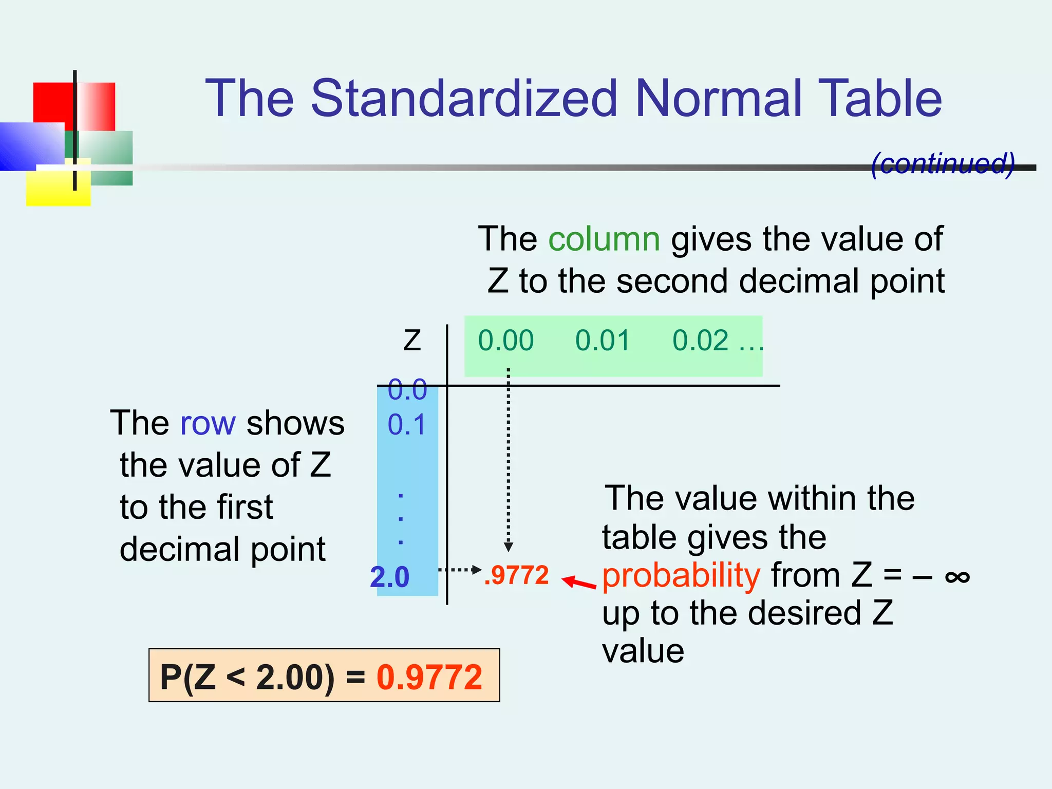
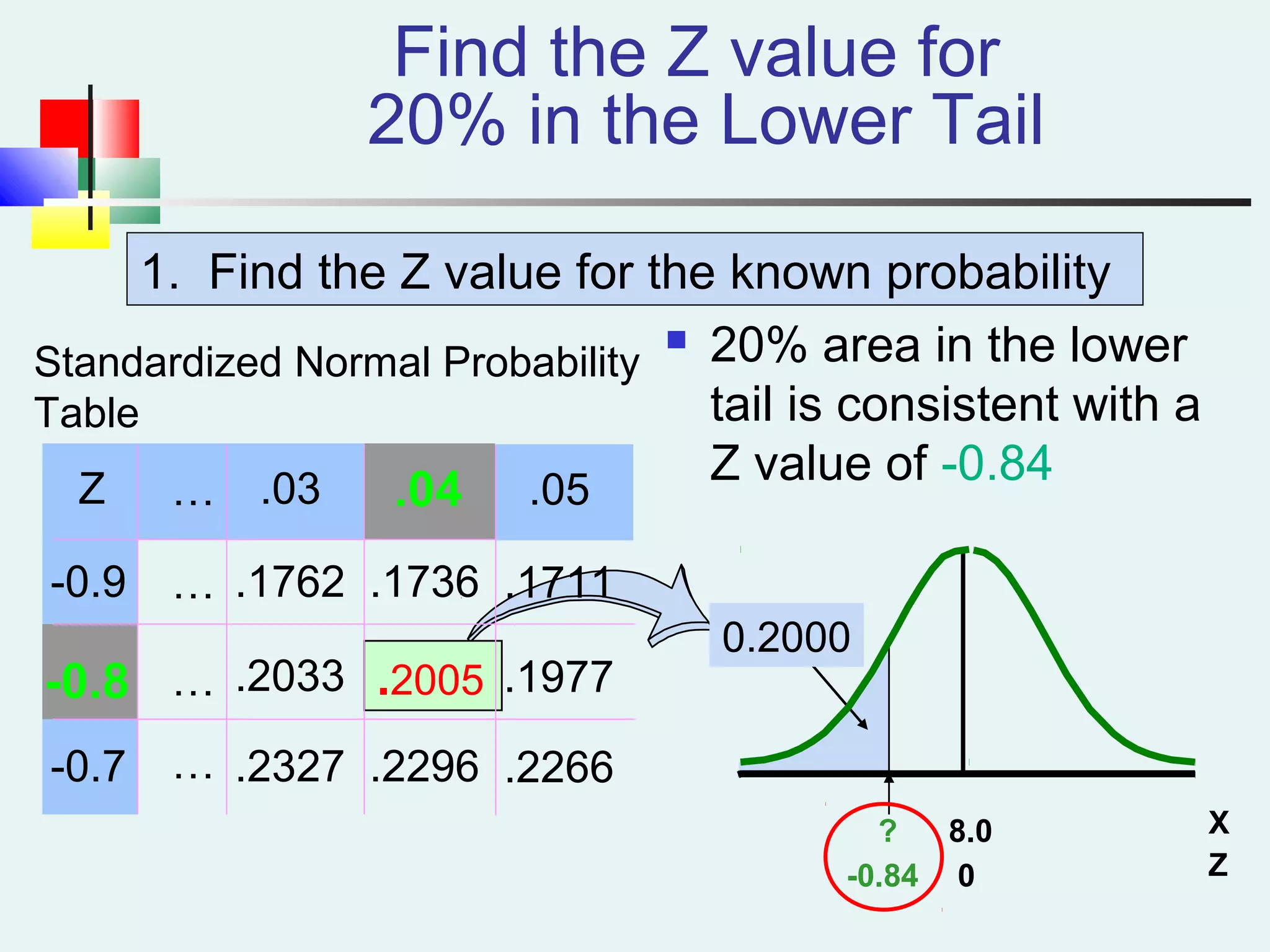
Understanding the transformation into standard normal distribution (Z), including Z-score calculations.
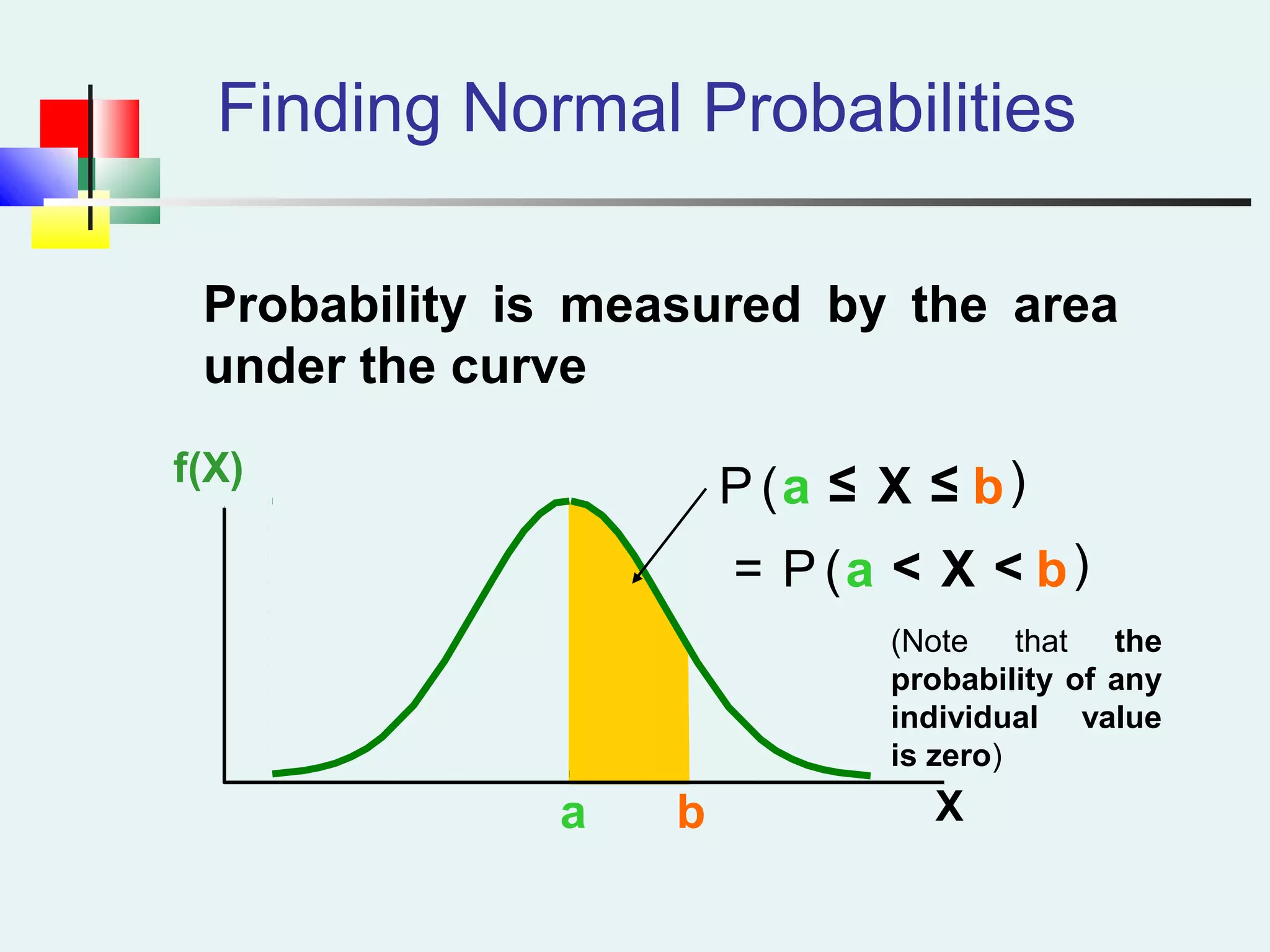
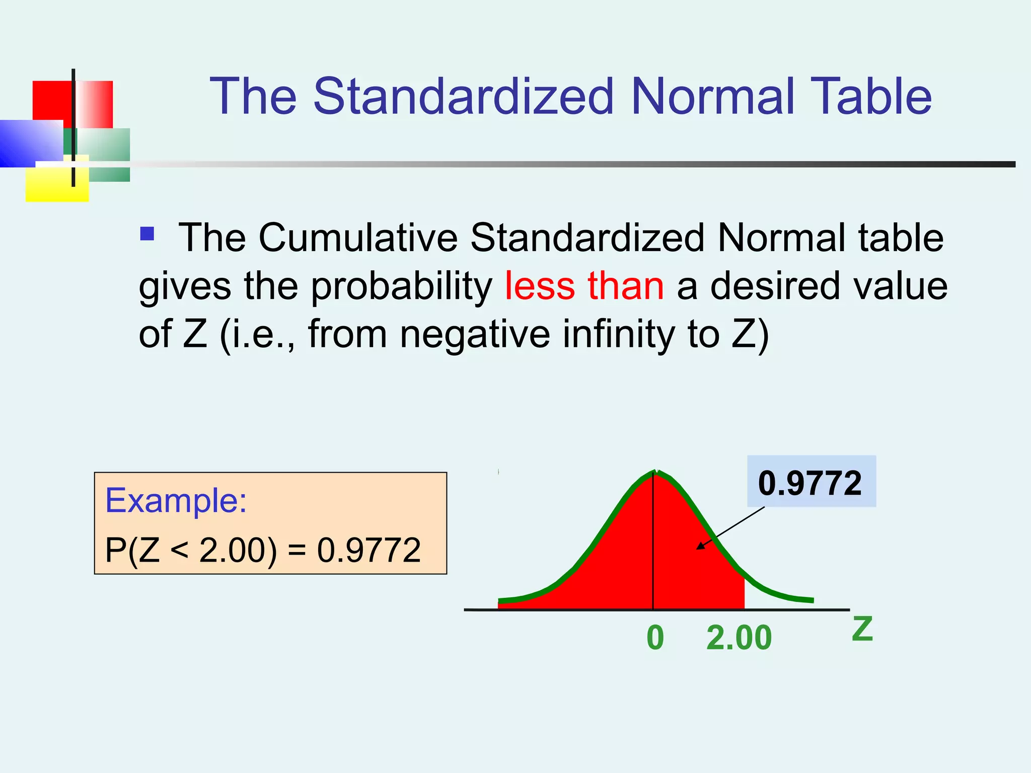
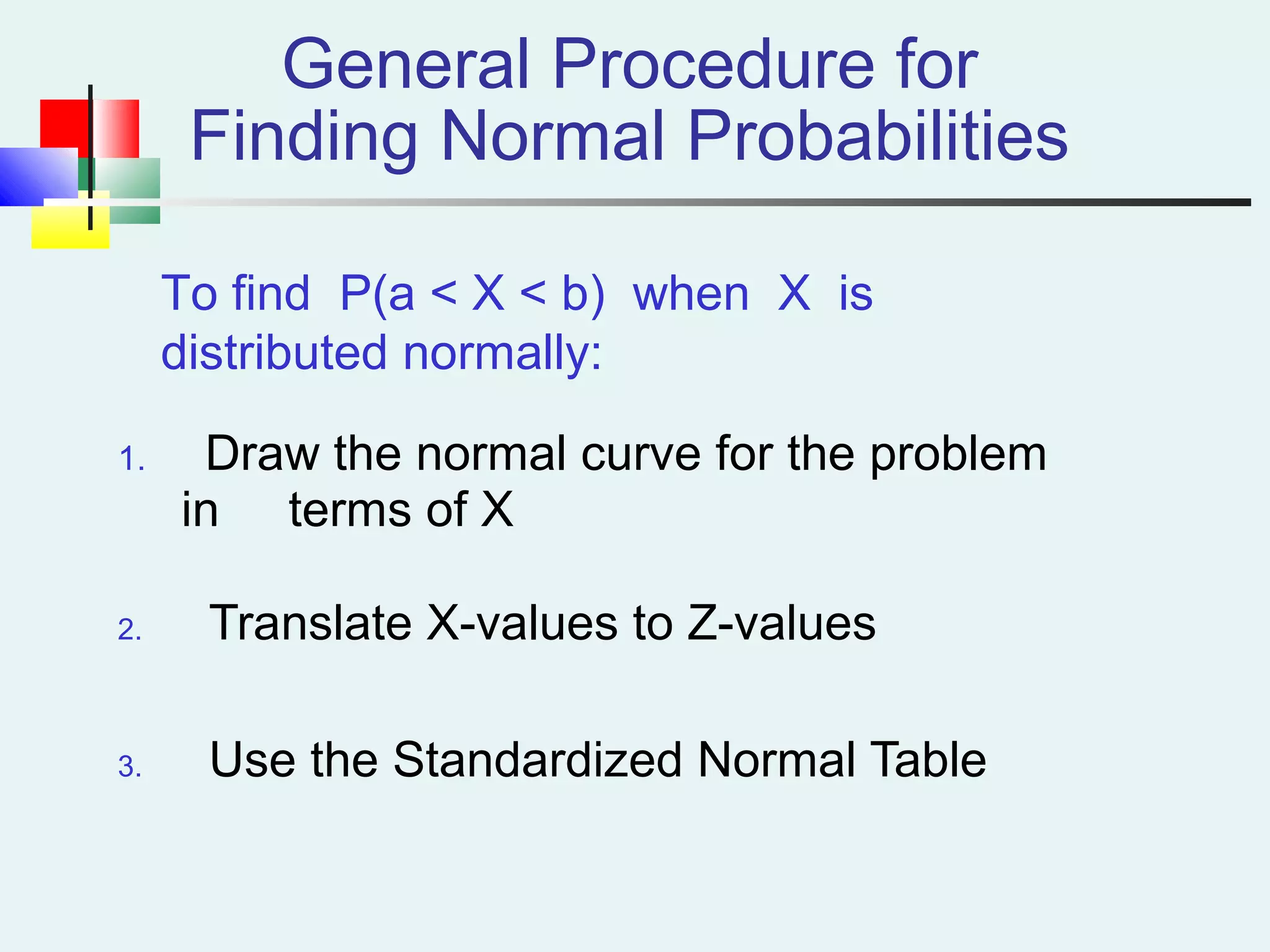
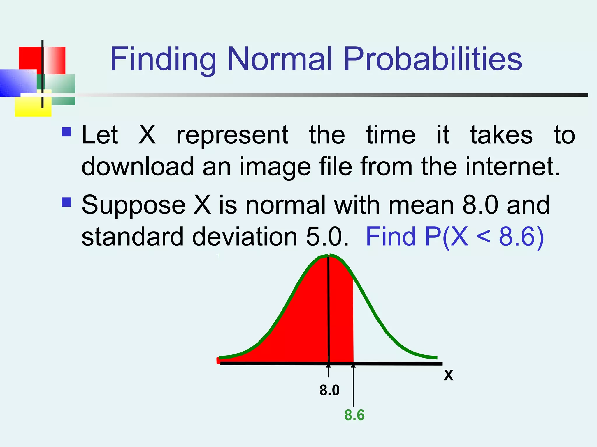
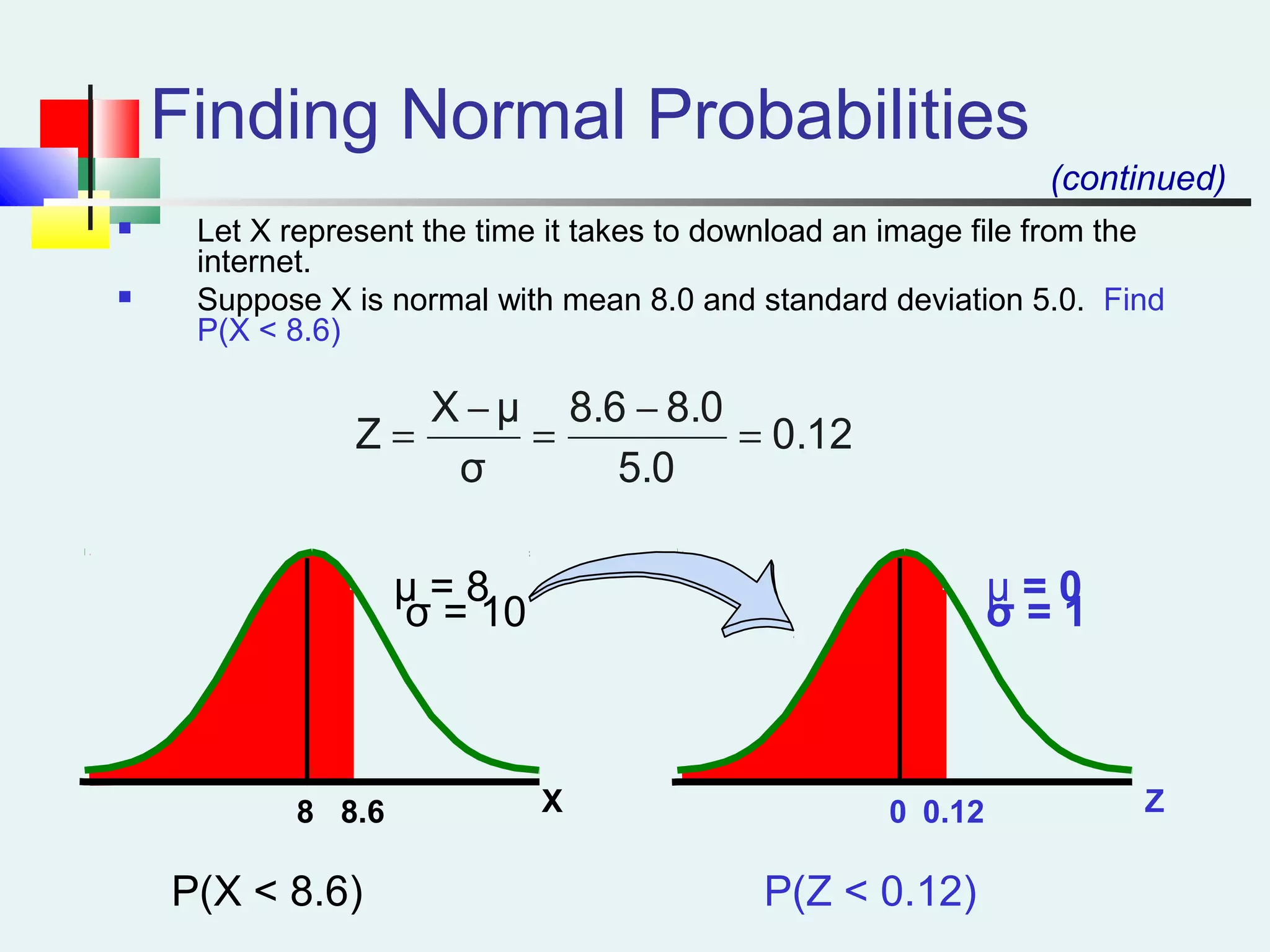
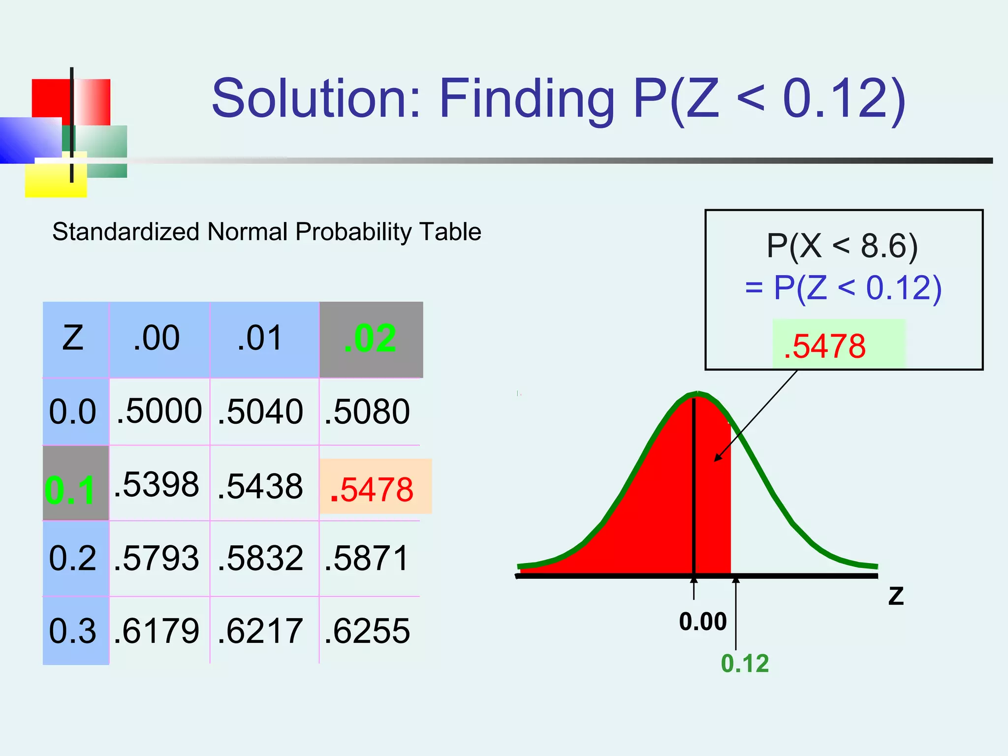
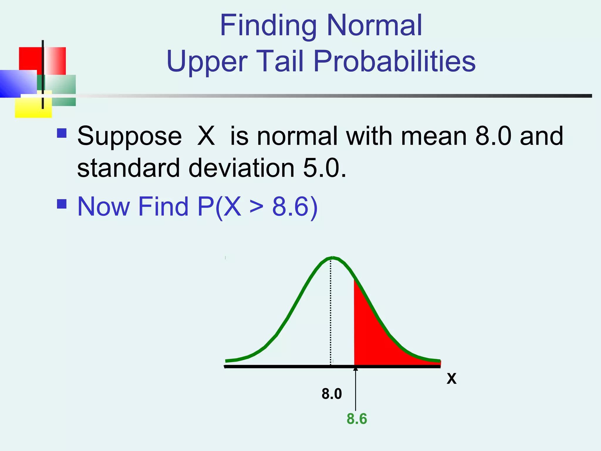
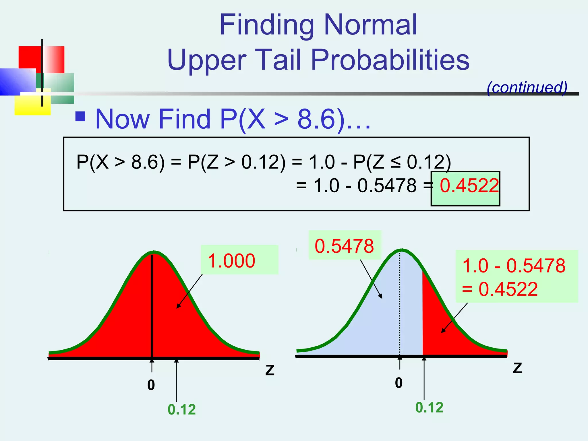
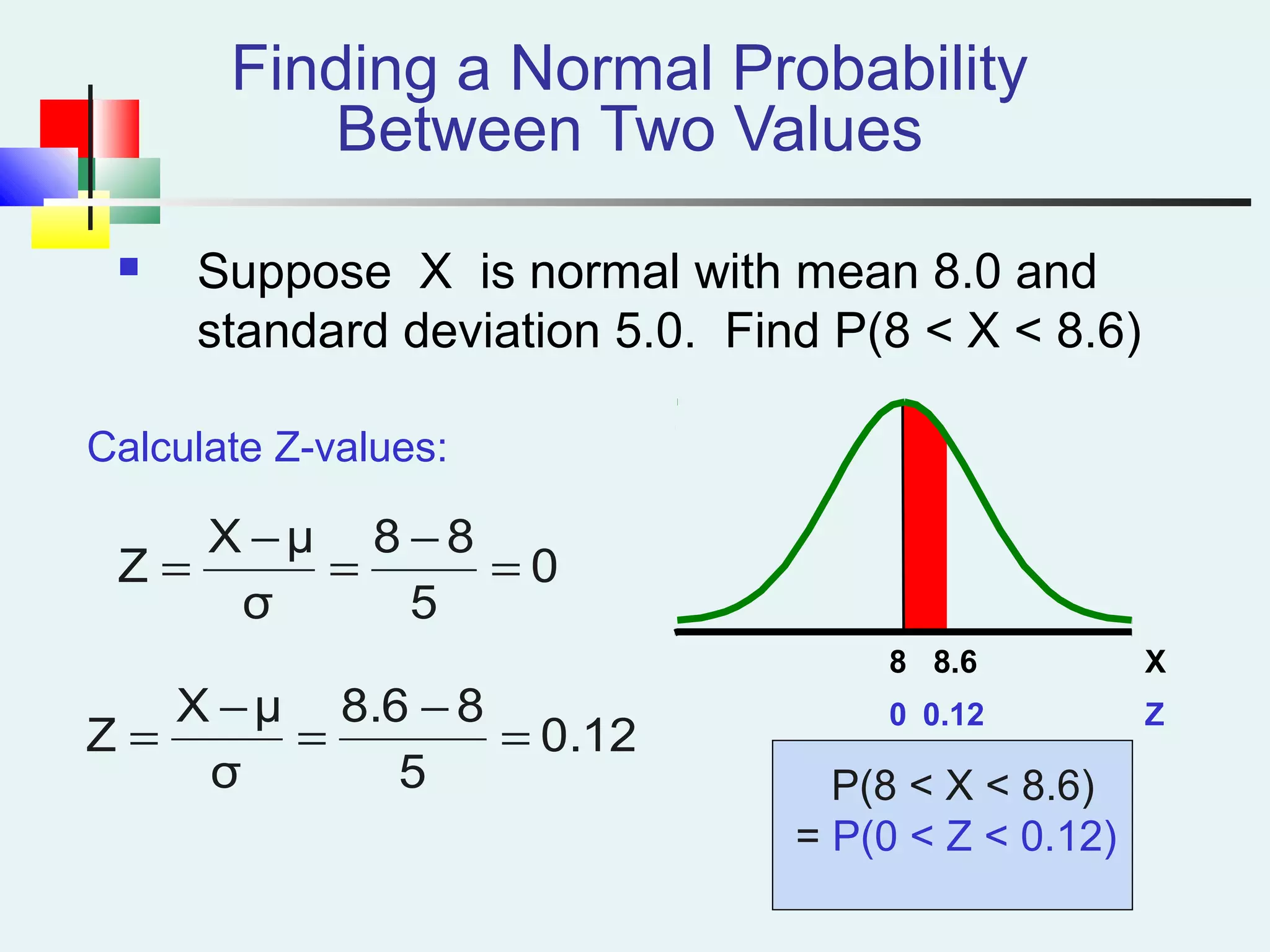
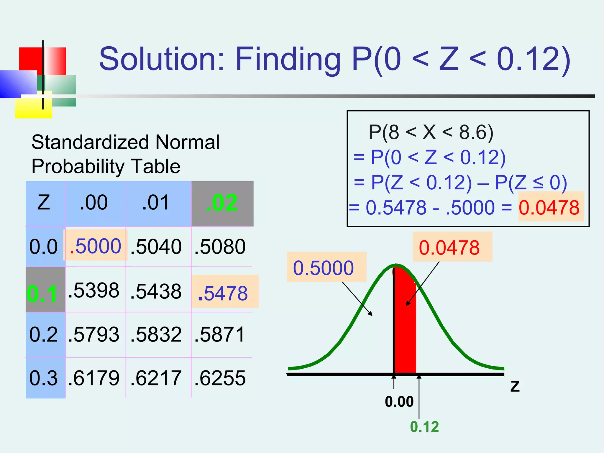
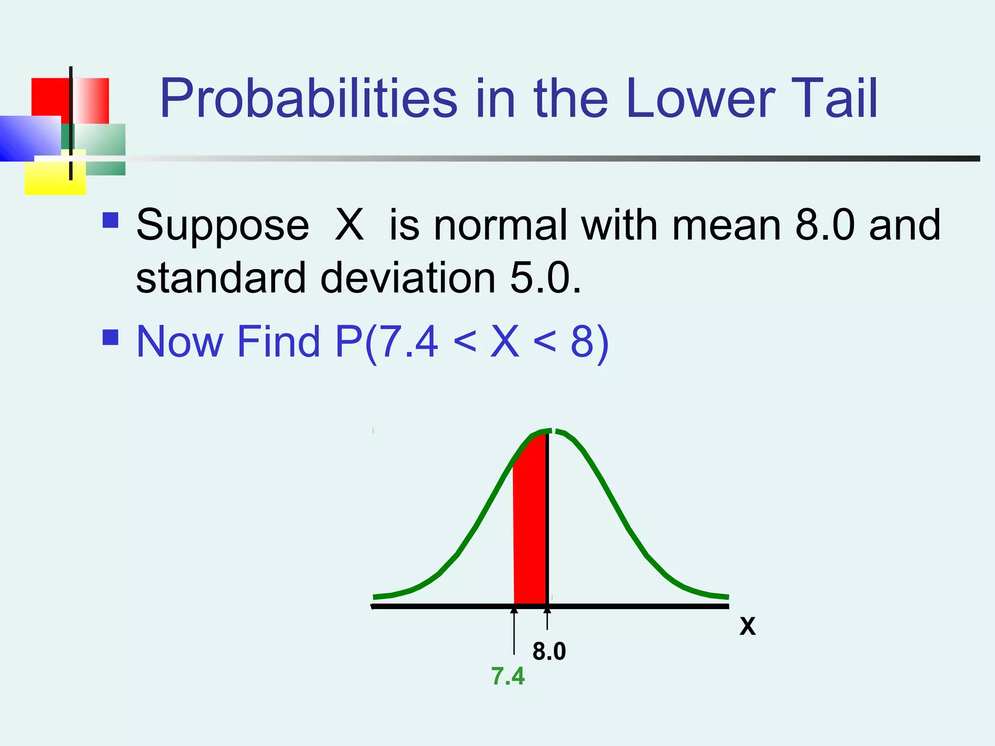
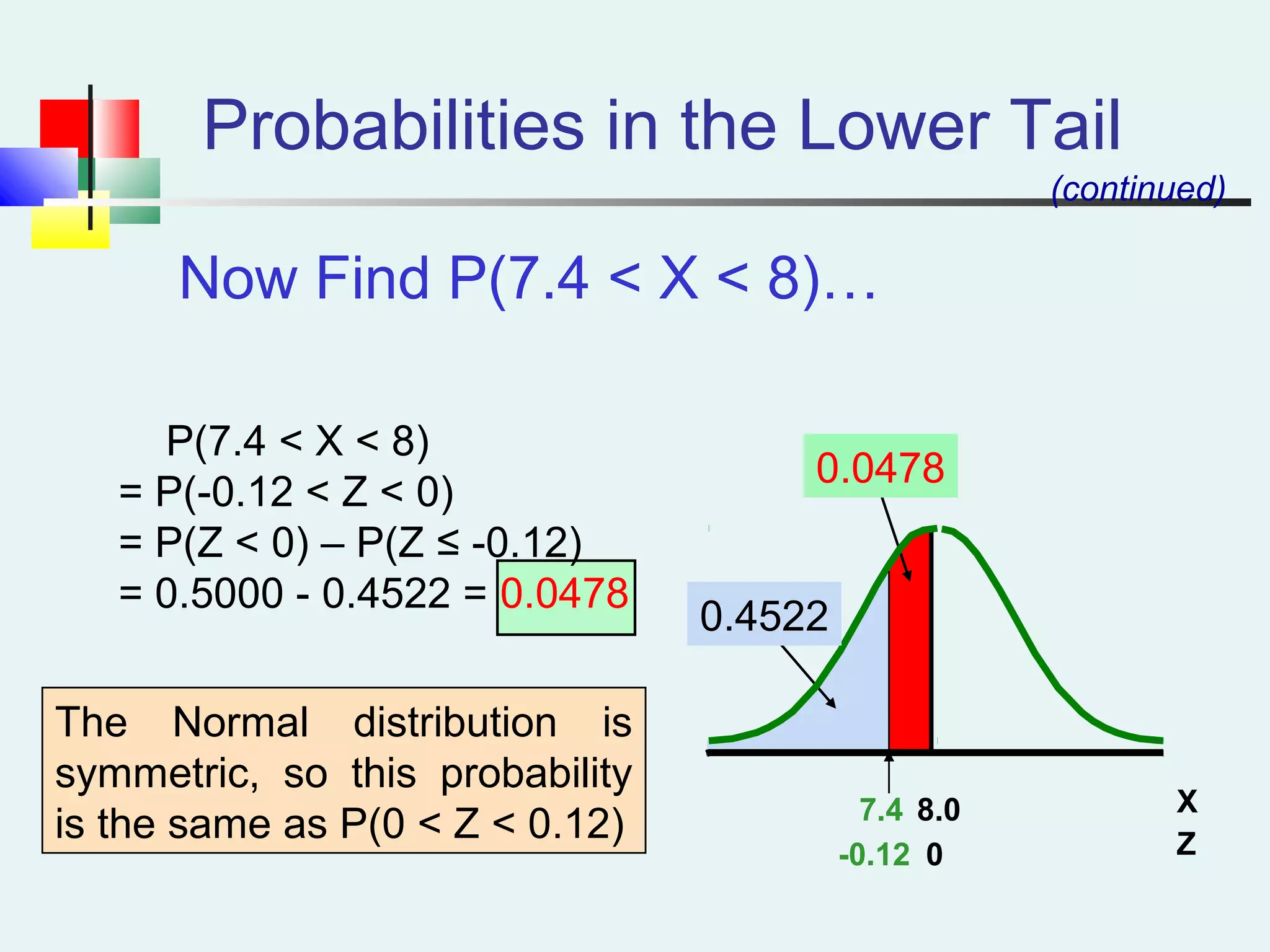
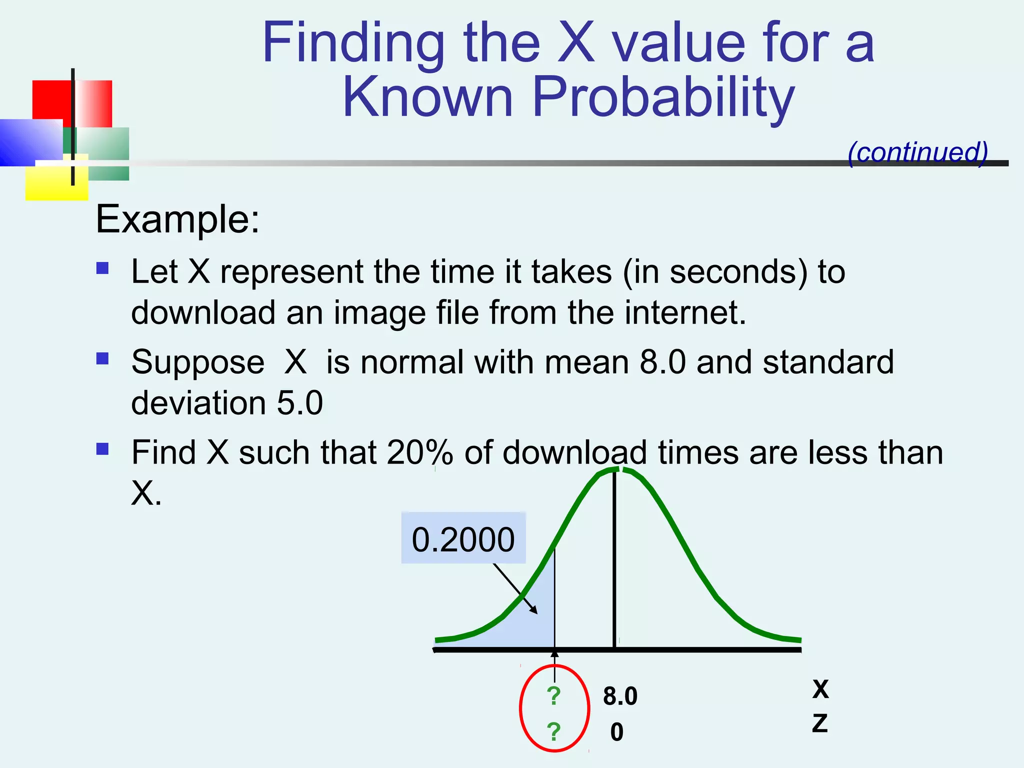
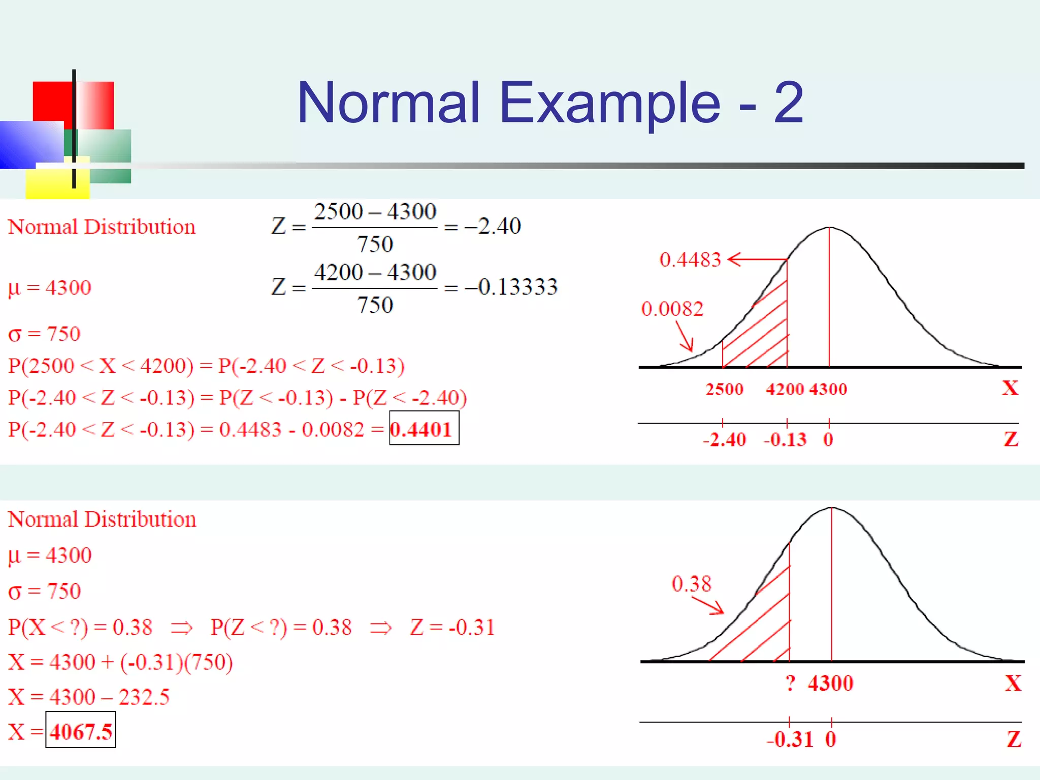
Finding probabilities for normal distributions using Z-scores and calculating areas under the curve.
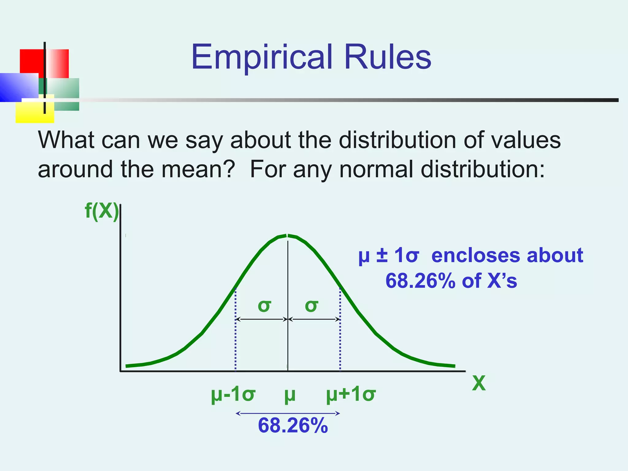
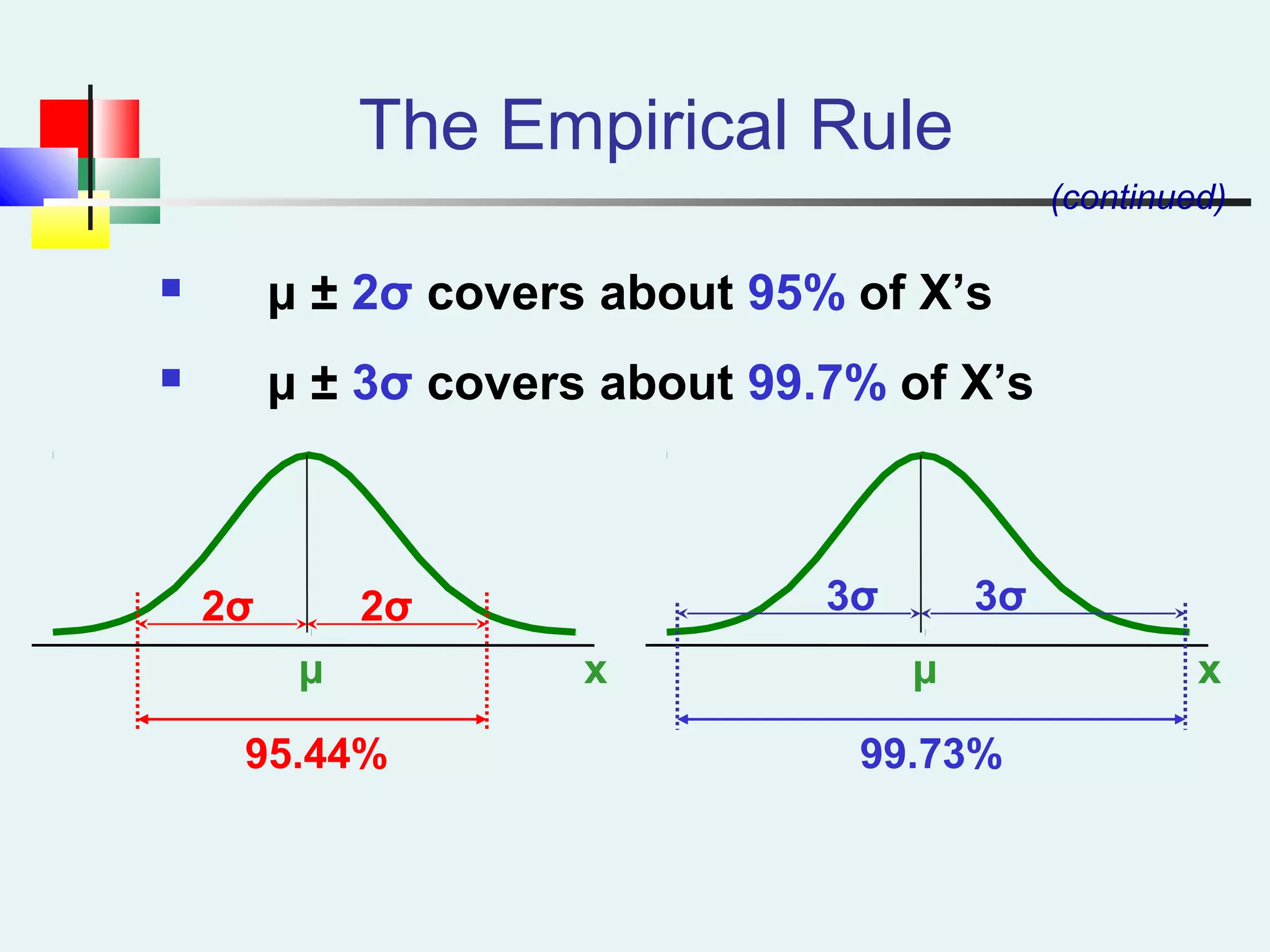
Explains the empirical rule applied to normal distributions, detailing coverage of data within standard deviations.
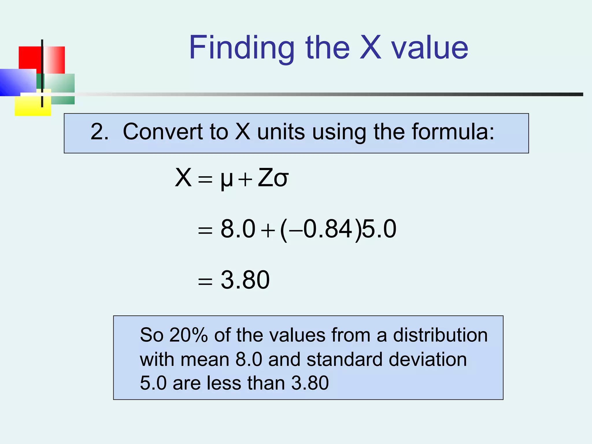
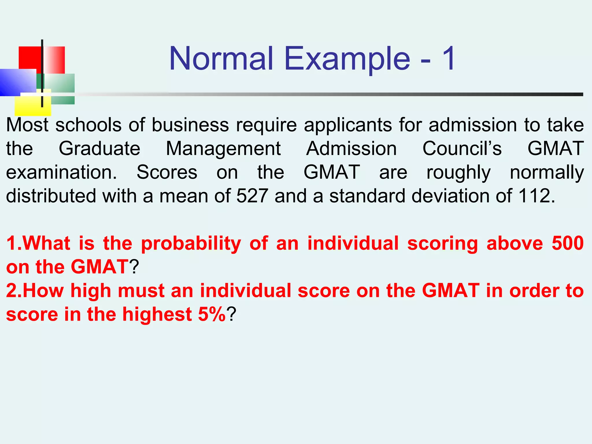
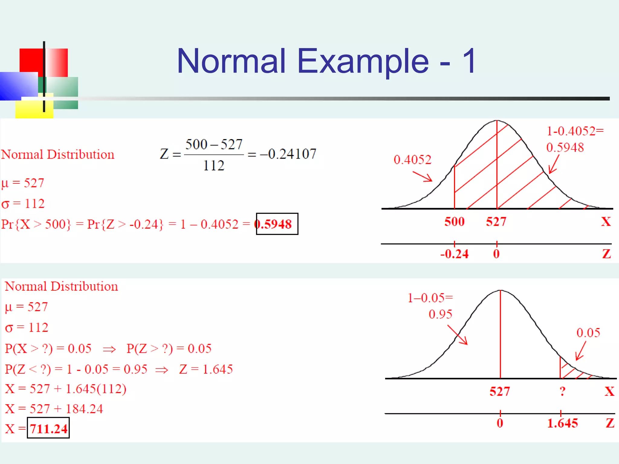
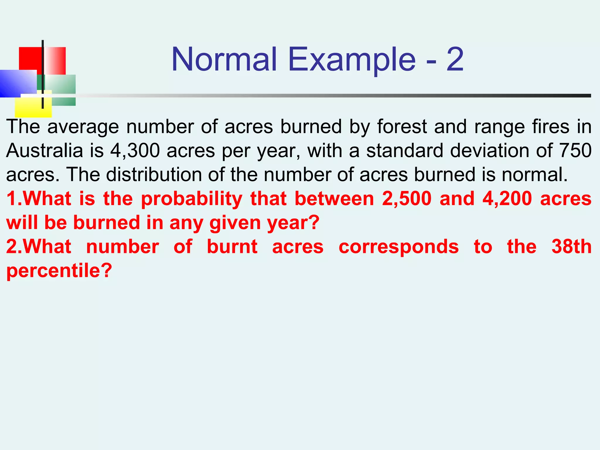
Examples using normal distributions in practical scenarios like GMAT scores and acres burned.


![[DSC Europe 25] Vid Stimac - Policy Parsimony: Between Oversimplifying and Ov...](https://cdn.slidesharecdn.com/ss_thumbnails/eqlepagzqp2rhg3gbluh-dsc-stimac-251120-251205090438-059e7f54-thumbnail.jpg?width=640&height=640&fit=bounds)
![[DSC Europe 25] Dragan Vucic - Building the Learning Organization - How AI Tr...](https://cdn.slidesharecdn.com/ss_thumbnails/8brigo2sbu6qur6gxrra-7-251205085715-6ae07d24-thumbnail.jpg?width=640&height=640&fit=bounds)


![[DSC Europe 25] Boris Perkovic - Lost in performance.pptx](https://cdn.slidesharecdn.com/ss_thumbnails/uq5hrp7vsuahqkxzifux-1-251204082258-fd2ee09d-thumbnail.jpg?width=640&height=640&fit=bounds)

![[DSC Europe 25] Petar Zivanov - AI meets documents From chatbots to AI-powere...](https://cdn.slidesharecdn.com/ss_thumbnails/xer2bb6nrdc8pdpev0pc-8-251204082258-7c2fa4a1-thumbnail.jpg?width=640&height=640&fit=bounds)
![[DSC Europe 25] Max Talanov - Non digital NNs.pptx](https://cdn.slidesharecdn.com/ss_thumbnails/wif8tr3gtua74qvtopke-non-digital-nns-251205090438-26b0eea6-thumbnail.jpg?width=640&height=640&fit=bounds)


