SlideShare a Scribd company logo
1 of 20
Example 1 – Vertical bar graphs

Bar graphs should be used when you are showing segments of information. From the
information given in the section on graph types, you will know that vertical bar graphs
are particularly useful for time series data. The space for labels on the x-axis is small,
but ideal for years, minutes, hours or months. At a glance you can see from the graph
that the scales for both the x- and y-axis increase as they get farther away from the
origin. Figure 1 below shows the number of police officers in Crimeville from 1993 to
2001.


In Figure 1 you can see that the number of police officers decreased from 1993 to 1996,
but started increasing again in 1996. The graph also makes it easy to compare or
contrast the number of police officers for any combination of years. For example, in
2001 there were nine more police officers than in 1998.

The double (or group) vertical bar graph is another effective means of comparing sets of
data about the same places or items. This type of vertical bar graph gives two or more
pieces of information for each item on the x-axis instead of just one as in Figure 1. This
allows you to make direct comparisons on the same graph by age group, sex, race, or
anything else you wish to compare. However, if a group vertical bar graph has too many
series of data, the graph becomes cluttered and it can be confusing to read.

Figure 2, a double vertical bar graph, compares two series of data: the numbers of boys
and girls using the Internet at Redwood Secondary School from 1995 to 2002. One bar
represents the number of boys who use the Internet and the other bar represents the
girls.
One disadvantage of vertical bar graphs, however, is that they lack space for text
labelling at the foot of each bar. When category labels in the graph are too long, you
might find a horizontal bar graph better for displaying information.


Example 2 – Horizontal bar graphs

The horizontal bar graph uses the y-axis (vertical line) for labelling. There is more room
to fit text labels for categorical variables on the y-axis.

Figure 3 shows the number of students at Diversity College who are immigrants by their
last country of permanent residence. The graph shows that 100 students immigrated
from China, 380 from France, and 260 from Brazil.

A horizontal bar graph has been used to show a comparison of these data. This graph is
the best method to present this type of information because the labels (in this case, the
countries' names) are too long to appear clearly on the x-axis.
A double or group horizontal bar graph is similar to a double or group vertical bar
graph, and it would be used when the labels are too long to fit on the x-axis.

In Figure 4, more than one piece of information is being delivered to the audience: drug
use by 15-year-old boys is being compared with drug use by 15-year-old girls at Jamie's
school. Having both pieces of information on the same graph makes it easier to
compare. The graph indicates that 32% of boys and 29% of girls have used hashish or
marijuana, and 3% of boys and 1% of girls have tried LSD. The graph also shows that
the same percent of boys and girls (4%) have used cocaine.


Example 3 – Comparing several places or items

Figure 5 is an example of a double horizontal bar graph. Hillary sampled an equal
number of boys and girls at her high school and asked them to pick the one snack food
they liked the most from the following list:

                           •   popcorn
                           •   chips
                           •   chocolate bars
                           •   crackers
                           •   pretzels
                           •   cookies
                           •   ice cream
                           •   fruit
                           •   candy
                           •   vegetables.

She created a graph to display the results of her survey. Examine Figure 5, and answer
the following questions:

                       1. What comparison does this graph show?
                       2. Which snack food was least preferred by girls?
                       3. Which snack food was preferred by substantially more
                          boys than girls?
                       4. Which snack foods were preferred by more girls than
                          boys?
5. Which snack food was preferred equally by both boys and
                         girls?


Answers

                      1. The graph shows a comparison of snack food preferences
                         by sex.
                      2. Vegetables were the snack food least preferred by girls.
                      3. A substantial number of more boys than girls preferred
                         chips.
                      4. Girls preferred candy, crackers, fruit and ice cream more
                         than boys did.
                      5. The same number of boys and girls preferred popcorn as
                         their snack food choice.


Example 4 – Inappropriate use of bar graphs

Vertical bar graphs are an excellent choice to emphasize a change in magnitude. The
best information for a vertical bar graph is data dealing with the description of
components, frequency distribution and time-series statistics.

A horizontal bar graph may be more effective than a line graph when there are fewer
time periods or segments of data. If you want to compare more than 9 or 10 items, use
a line graph instead. Figure 6 is an example of when a line graph should be used
instead of a horizontal bar graph.
Example 5 – Other bar graphs

There are several other types of bar graphs that you may encounter. The population
pyramid is a special application of a double bar graph. The following examples are rarely
used, but can be useful if used correctly.

Stacked bar graphs

The stacked bar graph is a preliminary data analysis tool used to show segments of
totals. Statistics Canada rarely uses them, despite the fact that stacked bar graphs can
convey a lot of information. The stacked bar graph can be very difficult to analyse if too
many items are in each stack. It can contrast values, but not necessarily in the simplest
manner.

In Figure 7, it is not difficult to analyse the data presented since there are only three
items in each stack: swimming, running and biking. It is easy to see at a glance what
percentage of time each woman spent on an event. Had this been a graph representing
a decathlon (with 10 events) the data would have been significantly harder to analyse.
Another reason that these graphs are rarely used is that they can represent a picture
other than the one that was intended. In the example above, it may have taken
Bronwyn two hours to finish the triathlon, and Rosalyn three hours, but they spent
almost the same percentage of time on each event. Both women spent 30% of their
times swimming, but whereas Rosalyn spent 54 minutes swimming, Bronwyn spent
36 minutes swimming. In other words, this graph does not tell you anything about their
ranking, only what percentage of their individual race times were spent on each event.
This can be misleading for someone who does not read the graph carefully.

Horizontal, vertical and stacked bar graph guidelines

You should keep the following guidelines in mind when creating your own bar graphs:

   •   Make bars and columns wider than the space between them.
   •   Do not allow grid lines to pass through columns or bars.
   •   Use a single font type on a graph. Try to maintain a consistent font style from
       graph to graph in a single presentation or document. Simple sans-serif fonts are
       preferable.
   •   Order your shade pattern from darkest to lightest on stacked bar graphs.
   •   Avoid garish colours or patterns.


Dot graphs

A dot graph is one of the simplest ways to represent information pictorially, yet it is the
graph that is least used. Figure 8 is an example of a dot graph. As you can see, the
message and the information behind the graph are delivered quickly and easily to the
reader.
Pie charts
   •   Constructing a pie chart
   •   Pie charts versus bar graphs

A pie chart is a way of summarizing a set of categorical data or displaying the different
values of a given variable (e.g., percentage distribution). This type of chart is a circle
divided into a series of segments. Each segment represents a particular category. The
area of each segment is the same proportion of a circle as the category is of the total
data set.

Pie charts usually show the component parts of a whole. Often you will see a segment
of the drawing separated from the rest of the pie in order to emphasize an important
piece of information.
The pie chart above clearly shows that 90% of all students and faculty members at
Avenue High School do not want to have a uniform dress code and that only 10% of the
school population would like to adopt school uniforms. This point is clearly emphasized
by its visual separation from the rest of the pie.

The use of the pie chart is quite popular, as the circle provides a visual concept of the
whole (100%). Pie charts are also one of the most commonly used charts because they
are simple to use. Despite its popularity, pie charts should be used sparingly for two
reasons. First, they are best used for displaying statistical information when there are
no more than six components only—otherwise, the resulting picture will be too complex
to understand. Second, pie charts are not useful when the values of each component
are similar because it is difficult to see the differences between slice sizes.

A pie chart uses percentages to compare information. Percentages are used because
they are the easiest way to represent a whole. The whole is equal to 100%. For
example, if you spend 7 hours at school and 55 minutes of that time is spent eating
lunch, then 13.1% of your school day was spent eating lunch. To present this in a pie
chart, you would need to find out how many degrees represent 13.1%. This calculation
is done by developing the equation:

percent ÷ 100 x 360 degrees = the number of degrees

This ratio works because the total percent of the pie chart represents 100% and there
are 360 degrees in a circle. Therefore 47.1 degrees of the circle (13.1%) represents the
time spent eating lunch.


Constructing a pie chart

A pie chart is constructed by converting the share of each component into a percentage
of 360 degrees. In Figure 2, music preferences in 14- to 19-year-olds are clearly shown.
The pie chart quickly tells you that

   •   half of students like rap best (50%), and
   •   the remaining students prefer alternative (25%), rock and roll (13%), country
       (10%) and classical (2%).

Tip! When drawing a pie chart, ensure that the segments are ordered by size (largest
to smallest) and in a clockwise direction.

In order to reproduce this pie chart, follow this step-by-step approach:

If 50% of the students liked rap, then 50% of the whole pie chart (360 degrees) would
equal 180 degrees.

1. Draw a circle with your protractor.
2. Starting from the 12 o'clock position on the circle, measure an angle of
   180 degrees with your protractor. The rap component should make up half of
   your circle. Mark this radius off with your ruler.
3. Repeat the process for each remaining music category, drawing in the radius
   according to its percentage of 360 degrees. The final category need not be
   measured as its radius is already in position.

Labeling the segments with percentage values often makes it easier to tell quickly which
segment is bigger. Whenever possible, the percentage and the category label should be
indicated beside their corresponding segments. This way, users do not have to
constantly look back at the legend in order to identify what category each colour
represents.
The pie chart above conveys a clear message to the user—that 88% of all students in
the World Religions class celebrate Easter. We can easily tell what the message is by
simply looking at the accompanying percentages. Unfortunately, the category labels are
too long to fit beside the pie segments, so they had to be placed in the legend. Ideally,
these labels would also accompany the pie segments.


It is more difficult to understand the message behind Figure 4 because there are no
percentage figures given for each slice of the pie. This is why it is important to label the
slices with actual values.

The user can still develop a picture of what is being said about the type of pets sold by
this store, but the message is not as clear as it would have been had the parts of the
pie been labelled.


In the pie chart above, the legend is formatted properly and the percentages are
included for each of the pie segments. However, there are too many items in the pie
chart to quickly give a clear picture of the distribution of movie genres. If there are
more than five or six categories, consider using a another graph to display the
information. Figure 5 would certainly be easier to read as a bar graph.
Tip! Many software programs will draw pie charts for you quickly and easily. However,
research has shown that many people can make mistakes when trying to compare pie
chart values. In general, bar graphs communicate the same message with less chance
for misunderstanding.


Pie charts versus bar graphs

When displaying statistical information, refrain from using more than one pie chart for
each figure.


Figure 6 shows two pie charts side-by-side, where a split bar graph (two bar graphs
back-to-back) would have shown the information more clearly. A user might find it
difficult to compare a segment from one pie chart to the corresponding segment of the
other pie chart. However, in a split bar graph, these segments become bars which are
lined up back-to-back, making it much easier to make comparisons.

Figure 7 shows how a split bar graph would be a better choice for displaying information
than a double pie chart. The key point in preparing this type of graph is to ensure that
you are using the same scale for both sides of the bar graph. You'll notice that the
information is much clearer in Figure 7 than in Figure 6.
Line graphs
   •   Comparing two related variables
   •   Multiple line graphs

Line graphs, especially useful in the fields of statistics and science, are more popular
than all other graphs combined because their visual characteristics reveal data trends
clearly and these graphs are easy to create.

A line graph is a visual comparison of how two variables—shown on the x- and y-axes—
are related or vary with each other. It shows related information by drawing a
continuous line between all the points on a grid. For information on the shapes of line
graphs, see the Organizing data chapter.

Line graphs compare two variables: one is plotted along the x-axis (horizontal) and the
other along the y-axis (vertical). The y-axis in a line graph usually indicates quantity
(e.g., dollars, litres) or percentage, while the horizontal x-axis often measures units of
time. As a result, the line graph is often viewed as a time series graph. For example, if
you wanted to graph the height of a baseball pitch over time, you could measure the
time variable along the x-axis, and the height along the y-axis.

Although they do not present specific data as well as tables do, line graphs are able to
show relationships more clearly than tables do. Line graphs can also depict multiple
series and hence are usually the best candidate for time series data and frequency
distribution.

Bar and column graphs and line graphs share a similar purpose. The column graph,
however, reveals a change in magnitude, whereas the line graph is used to show a
change in direction.

In summary, line graphs
•   show specific values of data well
   •   reveal trends and relationships between data
   •   compare trends in different groups of a variable

Graphs can give a distorted image of the data. If inconsistent scales on the axes of a
line graph force data to appear in a certain way, then a graph can even reveal a trend
that is entirely different from the one intended. This means that the intervals between
adjacent points along the axis may be dissimilar, or that the same data charted in two
graphs using different scales will appear different.


Example 1 – Plotting a trend over time

Figure 1 shows one obvious trend, the fluctuation in the labour force from January to
July. The number of students at Andrew's high school who are members of the labour
force is scaled using intervals on the y-axis, while the time variable is plotted on the x-
axis.

The number of students participating in the labour force was 252 in January, 252 in
February, 255 in March, 256 in April, 282 in May, 290 in June and 319 in July. When
examined further, the graph indicates that the labour force participation of these
students was at a plateau for the first four months covered by the graph (January to
April), and for the next three months (May to July) the number increased steadily.


Example 2 – Comparing two related variables

Figure 2 is a single line graph comparing two items; in this instance, time is not a
factor. The graph compares the number of dollars donated by the age of the donors.
According to the trend in the graph, the older the donor, the more money he or she
donates. The 17-year-old donors donate, on average, $84. For the 19-year-olds, the
average donation increased by $26 to make the average donation of that age group
$110.
Example 3 – Using correct scale

When drawing a line, it is important that you use the correct scale. Otherwise, the line's
shape can give readers the wrong impression about the data. Compare Figure 3 with
Figure 4:
Using a scale of 350 to 430 (Figure 3) focuses on a small range of values. It does not
accurately depict the trend in guilty crime offenders between January and May since it
exaggerates that trend and does not relate it to the bigger picture. However, choosing a
scale of 0 to 450 (Figure 4) better displays how small the decline in the number of guilty
crime offenders really was.


Example 4 – Multiple line graphs

A multiple line graph can effectively compare similar items over the same period of time
(Figure 5).


Figure 5 is an example of a very good graph. The message is clearly stated in the title,
and each of the line graphs is properly labelled. It is easy to see from this graph that
the total cell phone use has been rising steadily since 1996, except for a two-year
period (1999 and 2000) where the numbers drop slightly. The pattern of use for women
and men seems to be quite similar with very small discrepancies between them.


Scatterplots
•   Positive or direct relationships
   •   Scattered data points
   •   Data widely spread

In science, the scatterplot is widely used to present measurements of two or more
related variables. It is particularly useful when the variables of the y-axis are thought to
be dependent upon the values of the variable of the x-axis (usually an independent
variable).

In a scatterplot, the data points are plotted but not joined; the resulting pattern
indicates the type and strength of the relationship between two or more variables (see
Figure 1 below).


Car ownership increases as the household income increases, showing that there is a
positive relationship between these two variables.

The pattern of the data points on the scatterplot reveals the relationship between the
variables. Scatterplots can illustrate various patterns and relationships, such as:

   •   data correlation
   •   positive or direct relationships between variables
   •   negative or inverse relationships between variables
   •   scattered data points
   •   non-linear patterns
   •   spread of data
   •   outliers.


Data correlation

When the data points form a straight line on the graph, the linear relationship between
the variables is stronger and the correlation is higher (Figure 2).
Positive or direct relationships

If the points cluster around a line that runs from the lower left to upper right of the
graph area, then the relationship between the two variables is positive or direct
(Figure 3). An increase in the value of x is more likely associated with an increase in the
value of y. The closer the points are to the line, the stronger the relationship.


Negative or inverse relationships

If the points tend to cluster around a line that runs from the upper left to lower right of
the graph, then the relationship between the two variables is negative or inverse
(Figure 4).
Scattered data points

If the data points are randomly scattered, then there is no relationship between the two
variables; this means there is a low or zero correlation between the variables (Figure 5).


Non-linear patterns

Very low or zero correlation may result from a non-linear relationship between two
variables. If the relationship is, in fact, non-linear (i.e., points clustering around a curve,
not a straight line), the linear correlation coefficient will not be a good measure of the
strength of the relationship (Figure 6).
Spread of data

A scatterplot will also illustrate if the data are widely spread or if they are concentrated
within a smaller area (Figure 7 and 8).
Outliers

Besides portraying a non-linear relationship between the two variables, a scatterplot
can also show whether or not there exist any outliers in the data (Figure 9).

More Related Content

What's hot

Digital 2018 Philippines (January 2018)
Digital 2018 Philippines (January 2018)Digital 2018 Philippines (January 2018)
Digital 2018 Philippines (January 2018)DataReportal
 
The Hare-Hawes Cutting and Tydings-Mcduffie Law
The Hare-Hawes Cutting and Tydings-Mcduffie LawThe Hare-Hawes Cutting and Tydings-Mcduffie Law
The Hare-Hawes Cutting and Tydings-Mcduffie Lawruvyann
 
American Colonization Period in the Philippines (1901-1935)
American Colonization Period in the Philippines (1901-1935)American Colonization Period in the Philippines (1901-1935)
American Colonization Period in the Philippines (1901-1935)Shanish Asuncion
 
Philippine Presidents
Philippine PresidentsPhilippine Presidents
Philippine Presidentsschool
 
Aralin 20 ikalawang yugto ng himagsikang pilipino
Aralin 20 ikalawang yugto ng himagsikang pilipinoAralin 20 ikalawang yugto ng himagsikang pilipino
Aralin 20 ikalawang yugto ng himagsikang pilipinoChris Berandoy
 
506883677-Philippine-Agrarian-Reform.pdf
506883677-Philippine-Agrarian-Reform.pdf506883677-Philippine-Agrarian-Reform.pdf
506883677-Philippine-Agrarian-Reform.pdfLouieTemperante
 
Renaissance (dance)
Renaissance (dance)Renaissance (dance)
Renaissance (dance)hyagallenero
 
Fundamental positions of arms and feet
Fundamental positions of arms and feetFundamental positions of arms and feet
Fundamental positions of arms and feetIAn JoSeph VeLasco
 
B.-ELECTORAL-PROCESSES.pptx
B.-ELECTORAL-PROCESSES.pptxB.-ELECTORAL-PROCESSES.pptx
B.-ELECTORAL-PROCESSES.pptxjaneguinumtad3
 
Marcos Regime in the Philippines - Martial Law
Marcos Regime in the Philippines - Martial LawMarcos Regime in the Philippines - Martial Law
Marcos Regime in the Philippines - Martial LawIvan Bendiola
 
Foundation on Physical Education
 Foundation on Physical Education Foundation on Physical Education
Foundation on Physical EducationMayen Lobina
 
Personality check by jcnm.
Personality check by jcnm.Personality check by jcnm.
Personality check by jcnm.jhon carlo miras
 

What's hot (20)

American period
American periodAmerican period
American period
 
Digital 2018 Philippines (January 2018)
Digital 2018 Philippines (January 2018)Digital 2018 Philippines (January 2018)
Digital 2018 Philippines (January 2018)
 
The Hare-Hawes Cutting and Tydings-Mcduffie Law
The Hare-Hawes Cutting and Tydings-Mcduffie LawThe Hare-Hawes Cutting and Tydings-Mcduffie Law
The Hare-Hawes Cutting and Tydings-Mcduffie Law
 
American Colonization Period in the Philippines (1901-1935)
American Colonization Period in the Philippines (1901-1935)American Colonization Period in the Philippines (1901-1935)
American Colonization Period in the Philippines (1901-1935)
 
Swimming
SwimmingSwimming
Swimming
 
The Art of Philippine Films
The Art of Philippine FilmsThe Art of Philippine Films
The Art of Philippine Films
 
Philippine Presidents
Philippine PresidentsPhilippine Presidents
Philippine Presidents
 
Aralin 20 ikalawang yugto ng himagsikang pilipino
Aralin 20 ikalawang yugto ng himagsikang pilipinoAralin 20 ikalawang yugto ng himagsikang pilipino
Aralin 20 ikalawang yugto ng himagsikang pilipino
 
506883677-Philippine-Agrarian-Reform.pdf
506883677-Philippine-Agrarian-Reform.pdf506883677-Philippine-Agrarian-Reform.pdf
506883677-Philippine-Agrarian-Reform.pdf
 
Renaissance (dance)
Renaissance (dance)Renaissance (dance)
Renaissance (dance)
 
Fundamental positions of arms and feet
Fundamental positions of arms and feetFundamental positions of arms and feet
Fundamental positions of arms and feet
 
Cultural changes ang identity
Cultural changes ang identityCultural changes ang identity
Cultural changes ang identity
 
Aralin 15
Aralin 15Aralin 15
Aralin 15
 
B.-ELECTORAL-PROCESSES.pptx
B.-ELECTORAL-PROCESSES.pptxB.-ELECTORAL-PROCESSES.pptx
B.-ELECTORAL-PROCESSES.pptx
 
Marcos Regime in the Philippines - Martial Law
Marcos Regime in the Philippines - Martial LawMarcos Regime in the Philippines - Martial Law
Marcos Regime in the Philippines - Martial Law
 
Dance
DanceDance
Dance
 
Foundation on Physical Education
 Foundation on Physical Education Foundation on Physical Education
Foundation on Physical Education
 
GOV'T POLICIES.pptx
GOV'T POLICIES.pptxGOV'T POLICIES.pptx
GOV'T POLICIES.pptx
 
BROCHURE FOR BBM.pptx
BROCHURE FOR BBM.pptxBROCHURE FOR BBM.pptx
BROCHURE FOR BBM.pptx
 
Personality check by jcnm.
Personality check by jcnm.Personality check by jcnm.
Personality check by jcnm.
 

Viewers also liked

Chapter 4 260110 044531
Chapter 4 260110 044531Chapter 4 260110 044531
Chapter 4 260110 044531guest25d353
 
First finals examination
First finals examinationFirst finals examination
First finals examinationmyemeyegranil
 
Chapter 2 250110 083240
Chapter 2 250110 083240Chapter 2 250110 083240
Chapter 2 250110 083240guest25d353
 
Chapter 3 260110 044503
Chapter 3 260110 044503Chapter 3 260110 044503
Chapter 3 260110 044503guest25d353
 
Grade 4 Math
Grade 4 MathGrade 4 Math
Grade 4 MathMiss l
 
Grade 4 mtap reviewer
Grade 4 mtap reviewerGrade 4 mtap reviewer
Grade 4 mtap reviewerEclud Sugar
 

Viewers also liked (6)

Chapter 4 260110 044531
Chapter 4 260110 044531Chapter 4 260110 044531
Chapter 4 260110 044531
 
First finals examination
First finals examinationFirst finals examination
First finals examination
 
Chapter 2 250110 083240
Chapter 2 250110 083240Chapter 2 250110 083240
Chapter 2 250110 083240
 
Chapter 3 260110 044503
Chapter 3 260110 044503Chapter 3 260110 044503
Chapter 3 260110 044503
 
Grade 4 Math
Grade 4 MathGrade 4 Math
Grade 4 Math
 
Grade 4 mtap reviewer
Grade 4 mtap reviewerGrade 4 mtap reviewer
Grade 4 mtap reviewer
 

Similar to GRAPH AND CHARTS

Chapter 4 Problem 31. For problem three in chapter four, a teac.docx
Chapter 4 Problem 31. For problem three in chapter four,   a teac.docxChapter 4 Problem 31. For problem three in chapter four,   a teac.docx
Chapter 4 Problem 31. For problem three in chapter four, a teac.docxrobertad6
 
Statistics
StatisticsStatistics
Statisticsdiereck
 
1.AdvantagesandDisadvantagesofDotPlotsHistogramsandBoxPlotsLesson.pptx
1.AdvantagesandDisadvantagesofDotPlotsHistogramsandBoxPlotsLesson.pptx1.AdvantagesandDisadvantagesofDotPlotsHistogramsandBoxPlotsLesson.pptx
1.AdvantagesandDisadvantagesofDotPlotsHistogramsandBoxPlotsLesson.pptxAayzazAhmad
 
Different Types of Graphs
Different Types of GraphsDifferent Types of Graphs
Different Types of GraphsRileyAntler
 
(8) Lesson 8.1
(8) Lesson 8.1(8) Lesson 8.1
(8) Lesson 8.1wzuri
 
Introduction to Data Visualization
Introduction to Data VisualizationIntroduction to Data Visualization
Introduction to Data VisualizationStephen Tracy
 
Chapter 9 Study Guide
Chapter 9 Study GuideChapter 9 Study Guide
Chapter 9 Study Guidewzuri
 
(7) Lesson 10.5
(7) Lesson 10.5(7) Lesson 10.5
(7) Lesson 10.5wzuri
 
4 CREATING GRAPHS A PICTURE REALLY IS WORTH A THOUSAND WORDS4 M.docx
4 CREATING GRAPHS A PICTURE REALLY IS WORTH A THOUSAND WORDS4 M.docx4 CREATING GRAPHS A PICTURE REALLY IS WORTH A THOUSAND WORDS4 M.docx
4 CREATING GRAPHS A PICTURE REALLY IS WORTH A THOUSAND WORDS4 M.docxgilbertkpeters11344
 
Data Handling
Data Handling Data Handling
Data Handling 75193
 
There are three kinds of lies
There are three kinds of liesThere are three kinds of lies
There are three kinds of liesgwsis
 
SHOW Lesson Plan
SHOW Lesson PlanSHOW Lesson Plan
SHOW Lesson PlanRick Hodges
 
Instructional Video Lesson.pptx
Instructional Video Lesson.pptxInstructional Video Lesson.pptx
Instructional Video Lesson.pptxJhoelKenneth
 
Analysing charts and graphics
Analysing charts and graphicsAnalysing charts and graphics
Analysing charts and graphicsŠkola Futura
 
Visual Information
Visual InformationVisual Information
Visual Informationfeueacmrq
 
4.5 collecting and analyzing data
4.5   collecting and analyzing data4.5   collecting and analyzing data
4.5 collecting and analyzing dataLeizelAlvarez1
 

Similar to GRAPH AND CHARTS (20)

Chapter 4 Problem 31. For problem three in chapter four, a teac.docx
Chapter 4 Problem 31. For problem three in chapter four,   a teac.docxChapter 4 Problem 31. For problem three in chapter four,   a teac.docx
Chapter 4 Problem 31. For problem three in chapter four, a teac.docx
 
Statistics
StatisticsStatistics
Statistics
 
1.AdvantagesandDisadvantagesofDotPlotsHistogramsandBoxPlotsLesson.pptx
1.AdvantagesandDisadvantagesofDotPlotsHistogramsandBoxPlotsLesson.pptx1.AdvantagesandDisadvantagesofDotPlotsHistogramsandBoxPlotsLesson.pptx
1.AdvantagesandDisadvantagesofDotPlotsHistogramsandBoxPlotsLesson.pptx
 
Org Disp Data
Org Disp DataOrg Disp Data
Org Disp Data
 
Different Types of Graphs
Different Types of GraphsDifferent Types of Graphs
Different Types of Graphs
 
(8) Lesson 8.1
(8) Lesson 8.1(8) Lesson 8.1
(8) Lesson 8.1
 
Introduction to Data Visualization
Introduction to Data VisualizationIntroduction to Data Visualization
Introduction to Data Visualization
 
Chapter 9 Study Guide
Chapter 9 Study GuideChapter 9 Study Guide
Chapter 9 Study Guide
 
(7) Lesson 10.5
(7) Lesson 10.5(7) Lesson 10.5
(7) Lesson 10.5
 
Bar Graph
Bar GraphBar Graph
Bar Graph
 
4 CREATING GRAPHS A PICTURE REALLY IS WORTH A THOUSAND WORDS4 M.docx
4 CREATING GRAPHS A PICTURE REALLY IS WORTH A THOUSAND WORDS4 M.docx4 CREATING GRAPHS A PICTURE REALLY IS WORTH A THOUSAND WORDS4 M.docx
4 CREATING GRAPHS A PICTURE REALLY IS WORTH A THOUSAND WORDS4 M.docx
 
Data Handling
Data Handling Data Handling
Data Handling
 
There are three kinds of lies
There are three kinds of liesThere are three kinds of lies
There are three kinds of lies
 
Statistics three
Statistics threeStatistics three
Statistics three
 
SHOW Lesson Plan
SHOW Lesson PlanSHOW Lesson Plan
SHOW Lesson Plan
 
Instructional Video Lesson.pptx
Instructional Video Lesson.pptxInstructional Video Lesson.pptx
Instructional Video Lesson.pptx
 
Analysing charts and graphics
Analysing charts and graphicsAnalysing charts and graphics
Analysing charts and graphics
 
Visual Information
Visual InformationVisual Information
Visual Information
 
Chap 03 03
Chap 03 03Chap 03 03
Chap 03 03
 
4.5 collecting and analyzing data
4.5   collecting and analyzing data4.5   collecting and analyzing data
4.5 collecting and analyzing data
 

More from Aprendamos Facil

Inglés Empresarial para Directivos--Business English-Granollers
Inglés Empresarial para Directivos--Business English-GranollersInglés Empresarial para Directivos--Business English-Granollers
Inglés Empresarial para Directivos--Business English-GranollersAprendamos Facil
 
2-INGLÉS -ELEMENTAL-NUMBERS-GRANOLLERS.wmv
2-INGLÉS -ELEMENTAL-NUMBERS-GRANOLLERS.wmv 2-INGLÉS -ELEMENTAL-NUMBERS-GRANOLLERS.wmv
2-INGLÉS -ELEMENTAL-NUMBERS-GRANOLLERS.wmv Aprendamos Facil
 
-CLASE DE INGLÉS REFUERZO DE LA ESO GRANOLLERS.wmv
-CLASE DE INGLÉS REFUERZO DE LA ESO GRANOLLERS.wmv -CLASE DE INGLÉS REFUERZO DE LA ESO GRANOLLERS.wmv
-CLASE DE INGLÉS REFUERZO DE LA ESO GRANOLLERS.wmv Aprendamos Facil
 
1 inglés-elemental- inflections-granollers
1 inglés-elemental- inflections-granollers1 inglés-elemental- inflections-granollers
1 inglés-elemental- inflections-granollersAprendamos Facil
 
1 clase de inglés refuerzo de la eso- granollers
1 clase de inglés  refuerzo de la eso- granollers1 clase de inglés  refuerzo de la eso- granollers
1 clase de inglés refuerzo de la eso- granollersAprendamos Facil
 
Débat francaise-nivel -a1 a
Débat francaise-nivel -a1 aDébat francaise-nivel -a1 a
Débat francaise-nivel -a1 aAprendamos Facil
 
Curso de francés - vocabulario
Curso de  francés - vocabularioCurso de  francés - vocabulario
Curso de francés - vocabularioAprendamos Facil
 
Actions, present continuous
Actions, present continuousActions, present continuous
Actions, present continuousAprendamos Facil
 
CANCIONES GRATUITAS EN INGLÉS-GRANOLLERS -BARCELONA
CANCIONES GRATUITAS EN INGLÉS-GRANOLLERS -BARCELONACANCIONES GRATUITAS EN INGLÉS-GRANOLLERS -BARCELONA
CANCIONES GRATUITAS EN INGLÉS-GRANOLLERS -BARCELONAAprendamos Facil
 
FRANCÉS ELEMENTAL -GRANOLLERS-BARCELONA
FRANCÉS ELEMENTAL -GRANOLLERS-BARCELONAFRANCÉS ELEMENTAL -GRANOLLERS-BARCELONA
FRANCÉS ELEMENTAL -GRANOLLERS-BARCELONAAprendamos Facil
 
CURSO DE INGLÉS GRATUITO -GRANOLLERS-BARCELONA
CURSO DE INGLÉS GRATUITO -GRANOLLERS-BARCELONACURSO DE INGLÉS GRATUITO -GRANOLLERS-BARCELONA
CURSO DE INGLÉS GRATUITO -GRANOLLERS-BARCELONAAprendamos Facil
 

More from Aprendamos Facil (20)

Inglés Empresarial para Directivos--Business English-Granollers
Inglés Empresarial para Directivos--Business English-GranollersInglés Empresarial para Directivos--Business English-Granollers
Inglés Empresarial para Directivos--Business English-Granollers
 
2-INGLÉS -ELEMENTAL-NUMBERS-GRANOLLERS.wmv
2-INGLÉS -ELEMENTAL-NUMBERS-GRANOLLERS.wmv 2-INGLÉS -ELEMENTAL-NUMBERS-GRANOLLERS.wmv
2-INGLÉS -ELEMENTAL-NUMBERS-GRANOLLERS.wmv
 
-CLASE DE INGLÉS REFUERZO DE LA ESO GRANOLLERS.wmv
-CLASE DE INGLÉS REFUERZO DE LA ESO GRANOLLERS.wmv -CLASE DE INGLÉS REFUERZO DE LA ESO GRANOLLERS.wmv
-CLASE DE INGLÉS REFUERZO DE LA ESO GRANOLLERS.wmv
 
1 inglés-elemental- inflections-granollers
1 inglés-elemental- inflections-granollers1 inglés-elemental- inflections-granollers
1 inglés-elemental- inflections-granollers
 
1 clase de inglés refuerzo de la eso- granollers
1 clase de inglés  refuerzo de la eso- granollers1 clase de inglés  refuerzo de la eso- granollers
1 clase de inglés refuerzo de la eso- granollers
 
Débat francaise-nivel -a1 a
Débat francaise-nivel -a1 aDébat francaise-nivel -a1 a
Débat francaise-nivel -a1 a
 
Curso de francés - vocabulario
Curso de  francés - vocabularioCurso de  francés - vocabulario
Curso de francés - vocabulario
 
Classroom objects
Classroom objectsClassroom objects
Classroom objects
 
Classroom2 flash
Classroom2 flashClassroom2 flash
Classroom2 flash
 
Classroom flash
Classroom flashClassroom flash
Classroom flash
 
Dailyroutines2 flash
Dailyroutines2 flashDailyroutines2 flash
Dailyroutines2 flash
 
Dailyroutines1 flash
Dailyroutines1 flashDailyroutines1 flash
Dailyroutines1 flash
 
Verbs1 flash
Verbs1 flashVerbs1 flash
Verbs1 flash
 
Actions, present continuous
Actions, present continuousActions, present continuous
Actions, present continuous
 
Diagrams
DiagramsDiagrams
Diagrams
 
Grammaire française
Grammaire françaiseGrammaire française
Grammaire française
 
CHART AND GRAPH
CHART AND GRAPHCHART AND GRAPH
CHART AND GRAPH
 
CANCIONES GRATUITAS EN INGLÉS-GRANOLLERS -BARCELONA
CANCIONES GRATUITAS EN INGLÉS-GRANOLLERS -BARCELONACANCIONES GRATUITAS EN INGLÉS-GRANOLLERS -BARCELONA
CANCIONES GRATUITAS EN INGLÉS-GRANOLLERS -BARCELONA
 
FRANCÉS ELEMENTAL -GRANOLLERS-BARCELONA
FRANCÉS ELEMENTAL -GRANOLLERS-BARCELONAFRANCÉS ELEMENTAL -GRANOLLERS-BARCELONA
FRANCÉS ELEMENTAL -GRANOLLERS-BARCELONA
 
CURSO DE INGLÉS GRATUITO -GRANOLLERS-BARCELONA
CURSO DE INGLÉS GRATUITO -GRANOLLERS-BARCELONACURSO DE INGLÉS GRATUITO -GRANOLLERS-BARCELONA
CURSO DE INGLÉS GRATUITO -GRANOLLERS-BARCELONA
 

Recently uploaded

Developer Data Modeling Mistakes: From Postgres to NoSQL
Developer Data Modeling Mistakes: From Postgres to NoSQLDeveloper Data Modeling Mistakes: From Postgres to NoSQL
Developer Data Modeling Mistakes: From Postgres to NoSQLScyllaDB
 
Advanced Test Driven-Development @ php[tek] 2024
Advanced Test Driven-Development @ php[tek] 2024Advanced Test Driven-Development @ php[tek] 2024
Advanced Test Driven-Development @ php[tek] 2024Scott Keck-Warren
 
AI as an Interface for Commercial Buildings
AI as an Interface for Commercial BuildingsAI as an Interface for Commercial Buildings
AI as an Interface for Commercial BuildingsMemoori
 
Gen AI in Business - Global Trends Report 2024.pdf
Gen AI in Business - Global Trends Report 2024.pdfGen AI in Business - Global Trends Report 2024.pdf
Gen AI in Business - Global Trends Report 2024.pdfAddepto
 
Commit 2024 - Secret Management made easy
Commit 2024 - Secret Management made easyCommit 2024 - Secret Management made easy
Commit 2024 - Secret Management made easyAlfredo García Lavilla
 
My Hashitalk Indonesia April 2024 Presentation
My Hashitalk Indonesia April 2024 PresentationMy Hashitalk Indonesia April 2024 Presentation
My Hashitalk Indonesia April 2024 PresentationRidwan Fadjar
 
Bun (KitWorks Team Study 노별마루 발표 2024.4.22)
Bun (KitWorks Team Study 노별마루 발표 2024.4.22)Bun (KitWorks Team Study 노별마루 발표 2024.4.22)
Bun (KitWorks Team Study 노별마루 발표 2024.4.22)Wonjun Hwang
 
WordPress Websites for Engineers: Elevate Your Brand
WordPress Websites for Engineers: Elevate Your BrandWordPress Websites for Engineers: Elevate Your Brand
WordPress Websites for Engineers: Elevate Your Brandgvaughan
 
New from BookNet Canada for 2024: BNC CataList - Tech Forum 2024
New from BookNet Canada for 2024: BNC CataList - Tech Forum 2024New from BookNet Canada for 2024: BNC CataList - Tech Forum 2024
New from BookNet Canada for 2024: BNC CataList - Tech Forum 2024BookNet Canada
 
Unraveling Multimodality with Large Language Models.pdf
Unraveling Multimodality with Large Language Models.pdfUnraveling Multimodality with Large Language Models.pdf
Unraveling Multimodality with Large Language Models.pdfAlex Barbosa Coqueiro
 
Vector Databases 101 - An introduction to the world of Vector Databases
Vector Databases 101 - An introduction to the world of Vector DatabasesVector Databases 101 - An introduction to the world of Vector Databases
Vector Databases 101 - An introduction to the world of Vector DatabasesZilliz
 
"Federated learning: out of reach no matter how close",Oleksandr Lapshyn
"Federated learning: out of reach no matter how close",Oleksandr Lapshyn"Federated learning: out of reach no matter how close",Oleksandr Lapshyn
"Federated learning: out of reach no matter how close",Oleksandr LapshynFwdays
 
Scanning the Internet for External Cloud Exposures via SSL Certs
Scanning the Internet for External Cloud Exposures via SSL CertsScanning the Internet for External Cloud Exposures via SSL Certs
Scanning the Internet for External Cloud Exposures via SSL CertsRizwan Syed
 
DevEX - reference for building teams, processes, and platforms
DevEX - reference for building teams, processes, and platformsDevEX - reference for building teams, processes, and platforms
DevEX - reference for building teams, processes, and platformsSergiu Bodiu
 
Leverage Zilliz Serverless - Up to 50X Saving for Your Vector Storage Cost
Leverage Zilliz Serverless - Up to 50X Saving for Your Vector Storage CostLeverage Zilliz Serverless - Up to 50X Saving for Your Vector Storage Cost
Leverage Zilliz Serverless - Up to 50X Saving for Your Vector Storage CostZilliz
 
Transcript: New from BookNet Canada for 2024: BNC CataList - Tech Forum 2024
Transcript: New from BookNet Canada for 2024: BNC CataList - Tech Forum 2024Transcript: New from BookNet Canada for 2024: BNC CataList - Tech Forum 2024
Transcript: New from BookNet Canada for 2024: BNC CataList - Tech Forum 2024BookNet Canada
 
The Future of Software Development - Devin AI Innovative Approach.pdf
The Future of Software Development - Devin AI Innovative Approach.pdfThe Future of Software Development - Devin AI Innovative Approach.pdf
The Future of Software Development - Devin AI Innovative Approach.pdfSeasiaInfotech2
 
Integration and Automation in Practice: CI/CD in Mule Integration and Automat...
Integration and Automation in Practice: CI/CD in Mule Integration and Automat...Integration and Automation in Practice: CI/CD in Mule Integration and Automat...
Integration and Automation in Practice: CI/CD in Mule Integration and Automat...Patryk Bandurski
 
Artificial intelligence in cctv survelliance.pptx
Artificial intelligence in cctv survelliance.pptxArtificial intelligence in cctv survelliance.pptx
Artificial intelligence in cctv survelliance.pptxhariprasad279825
 

Recently uploaded (20)

Developer Data Modeling Mistakes: From Postgres to NoSQL
Developer Data Modeling Mistakes: From Postgres to NoSQLDeveloper Data Modeling Mistakes: From Postgres to NoSQL
Developer Data Modeling Mistakes: From Postgres to NoSQL
 
Advanced Test Driven-Development @ php[tek] 2024
Advanced Test Driven-Development @ php[tek] 2024Advanced Test Driven-Development @ php[tek] 2024
Advanced Test Driven-Development @ php[tek] 2024
 
AI as an Interface for Commercial Buildings
AI as an Interface for Commercial BuildingsAI as an Interface for Commercial Buildings
AI as an Interface for Commercial Buildings
 
Gen AI in Business - Global Trends Report 2024.pdf
Gen AI in Business - Global Trends Report 2024.pdfGen AI in Business - Global Trends Report 2024.pdf
Gen AI in Business - Global Trends Report 2024.pdf
 
DMCC Future of Trade Web3 - Special Edition
DMCC Future of Trade Web3 - Special EditionDMCC Future of Trade Web3 - Special Edition
DMCC Future of Trade Web3 - Special Edition
 
Commit 2024 - Secret Management made easy
Commit 2024 - Secret Management made easyCommit 2024 - Secret Management made easy
Commit 2024 - Secret Management made easy
 
My Hashitalk Indonesia April 2024 Presentation
My Hashitalk Indonesia April 2024 PresentationMy Hashitalk Indonesia April 2024 Presentation
My Hashitalk Indonesia April 2024 Presentation
 
Bun (KitWorks Team Study 노별마루 발표 2024.4.22)
Bun (KitWorks Team Study 노별마루 발표 2024.4.22)Bun (KitWorks Team Study 노별마루 발표 2024.4.22)
Bun (KitWorks Team Study 노별마루 발표 2024.4.22)
 
WordPress Websites for Engineers: Elevate Your Brand
WordPress Websites for Engineers: Elevate Your BrandWordPress Websites for Engineers: Elevate Your Brand
WordPress Websites for Engineers: Elevate Your Brand
 
New from BookNet Canada for 2024: BNC CataList - Tech Forum 2024
New from BookNet Canada for 2024: BNC CataList - Tech Forum 2024New from BookNet Canada for 2024: BNC CataList - Tech Forum 2024
New from BookNet Canada for 2024: BNC CataList - Tech Forum 2024
 
Unraveling Multimodality with Large Language Models.pdf
Unraveling Multimodality with Large Language Models.pdfUnraveling Multimodality with Large Language Models.pdf
Unraveling Multimodality with Large Language Models.pdf
 
Vector Databases 101 - An introduction to the world of Vector Databases
Vector Databases 101 - An introduction to the world of Vector DatabasesVector Databases 101 - An introduction to the world of Vector Databases
Vector Databases 101 - An introduction to the world of Vector Databases
 
"Federated learning: out of reach no matter how close",Oleksandr Lapshyn
"Federated learning: out of reach no matter how close",Oleksandr Lapshyn"Federated learning: out of reach no matter how close",Oleksandr Lapshyn
"Federated learning: out of reach no matter how close",Oleksandr Lapshyn
 
Scanning the Internet for External Cloud Exposures via SSL Certs
Scanning the Internet for External Cloud Exposures via SSL CertsScanning the Internet for External Cloud Exposures via SSL Certs
Scanning the Internet for External Cloud Exposures via SSL Certs
 
DevEX - reference for building teams, processes, and platforms
DevEX - reference for building teams, processes, and platformsDevEX - reference for building teams, processes, and platforms
DevEX - reference for building teams, processes, and platforms
 
Leverage Zilliz Serverless - Up to 50X Saving for Your Vector Storage Cost
Leverage Zilliz Serverless - Up to 50X Saving for Your Vector Storage CostLeverage Zilliz Serverless - Up to 50X Saving for Your Vector Storage Cost
Leverage Zilliz Serverless - Up to 50X Saving for Your Vector Storage Cost
 
Transcript: New from BookNet Canada for 2024: BNC CataList - Tech Forum 2024
Transcript: New from BookNet Canada for 2024: BNC CataList - Tech Forum 2024Transcript: New from BookNet Canada for 2024: BNC CataList - Tech Forum 2024
Transcript: New from BookNet Canada for 2024: BNC CataList - Tech Forum 2024
 
The Future of Software Development - Devin AI Innovative Approach.pdf
The Future of Software Development - Devin AI Innovative Approach.pdfThe Future of Software Development - Devin AI Innovative Approach.pdf
The Future of Software Development - Devin AI Innovative Approach.pdf
 
Integration and Automation in Practice: CI/CD in Mule Integration and Automat...
Integration and Automation in Practice: CI/CD in Mule Integration and Automat...Integration and Automation in Practice: CI/CD in Mule Integration and Automat...
Integration and Automation in Practice: CI/CD in Mule Integration and Automat...
 
Artificial intelligence in cctv survelliance.pptx
Artificial intelligence in cctv survelliance.pptxArtificial intelligence in cctv survelliance.pptx
Artificial intelligence in cctv survelliance.pptx
 

GRAPH AND CHARTS

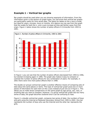
  • 1. Example 1 – Vertical bar graphs Bar graphs should be used when you are showing segments of information. From the information given in the section on graph types, you will know that vertical bar graphs are particularly useful for time series data. The space for labels on the x-axis is small, but ideal for years, minutes, hours or months. At a glance you can see from the graph that the scales for both the x- and y-axis increase as they get farther away from the origin. Figure 1 below shows the number of police officers in Crimeville from 1993 to 2001. In Figure 1 you can see that the number of police officers decreased from 1993 to 1996, but started increasing again in 1996. The graph also makes it easy to compare or contrast the number of police officers for any combination of years. For example, in 2001 there were nine more police officers than in 1998. The double (or group) vertical bar graph is another effective means of comparing sets of data about the same places or items. This type of vertical bar graph gives two or more pieces of information for each item on the x-axis instead of just one as in Figure 1. This allows you to make direct comparisons on the same graph by age group, sex, race, or anything else you wish to compare. However, if a group vertical bar graph has too many series of data, the graph becomes cluttered and it can be confusing to read. Figure 2, a double vertical bar graph, compares two series of data: the numbers of boys and girls using the Internet at Redwood Secondary School from 1995 to 2002. One bar represents the number of boys who use the Internet and the other bar represents the girls.
  • 2. One disadvantage of vertical bar graphs, however, is that they lack space for text labelling at the foot of each bar. When category labels in the graph are too long, you might find a horizontal bar graph better for displaying information. Example 2 – Horizontal bar graphs The horizontal bar graph uses the y-axis (vertical line) for labelling. There is more room to fit text labels for categorical variables on the y-axis. Figure 3 shows the number of students at Diversity College who are immigrants by their last country of permanent residence. The graph shows that 100 students immigrated from China, 380 from France, and 260 from Brazil. A horizontal bar graph has been used to show a comparison of these data. This graph is the best method to present this type of information because the labels (in this case, the countries' names) are too long to appear clearly on the x-axis.
  • 3. A double or group horizontal bar graph is similar to a double or group vertical bar graph, and it would be used when the labels are too long to fit on the x-axis. In Figure 4, more than one piece of information is being delivered to the audience: drug use by 15-year-old boys is being compared with drug use by 15-year-old girls at Jamie's school. Having both pieces of information on the same graph makes it easier to compare. The graph indicates that 32% of boys and 29% of girls have used hashish or marijuana, and 3% of boys and 1% of girls have tried LSD. The graph also shows that the same percent of boys and girls (4%) have used cocaine. Example 3 – Comparing several places or items Figure 5 is an example of a double horizontal bar graph. Hillary sampled an equal number of boys and girls at her high school and asked them to pick the one snack food they liked the most from the following list: • popcorn • chips • chocolate bars • crackers • pretzels • cookies • ice cream • fruit • candy • vegetables. She created a graph to display the results of her survey. Examine Figure 5, and answer the following questions: 1. What comparison does this graph show? 2. Which snack food was least preferred by girls? 3. Which snack food was preferred by substantially more boys than girls? 4. Which snack foods were preferred by more girls than boys?
  • 4. 5. Which snack food was preferred equally by both boys and girls? Answers 1. The graph shows a comparison of snack food preferences by sex. 2. Vegetables were the snack food least preferred by girls. 3. A substantial number of more boys than girls preferred chips. 4. Girls preferred candy, crackers, fruit and ice cream more than boys did. 5. The same number of boys and girls preferred popcorn as their snack food choice. Example 4 – Inappropriate use of bar graphs Vertical bar graphs are an excellent choice to emphasize a change in magnitude. The best information for a vertical bar graph is data dealing with the description of components, frequency distribution and time-series statistics. A horizontal bar graph may be more effective than a line graph when there are fewer time periods or segments of data. If you want to compare more than 9 or 10 items, use a line graph instead. Figure 6 is an example of when a line graph should be used instead of a horizontal bar graph.
  • 5. Example 5 – Other bar graphs There are several other types of bar graphs that you may encounter. The population pyramid is a special application of a double bar graph. The following examples are rarely used, but can be useful if used correctly. Stacked bar graphs The stacked bar graph is a preliminary data analysis tool used to show segments of totals. Statistics Canada rarely uses them, despite the fact that stacked bar graphs can convey a lot of information. The stacked bar graph can be very difficult to analyse if too many items are in each stack. It can contrast values, but not necessarily in the simplest manner. In Figure 7, it is not difficult to analyse the data presented since there are only three items in each stack: swimming, running and biking. It is easy to see at a glance what percentage of time each woman spent on an event. Had this been a graph representing a decathlon (with 10 events) the data would have been significantly harder to analyse.
  • 6. Another reason that these graphs are rarely used is that they can represent a picture other than the one that was intended. In the example above, it may have taken Bronwyn two hours to finish the triathlon, and Rosalyn three hours, but they spent almost the same percentage of time on each event. Both women spent 30% of their times swimming, but whereas Rosalyn spent 54 minutes swimming, Bronwyn spent 36 minutes swimming. In other words, this graph does not tell you anything about their ranking, only what percentage of their individual race times were spent on each event. This can be misleading for someone who does not read the graph carefully. Horizontal, vertical and stacked bar graph guidelines You should keep the following guidelines in mind when creating your own bar graphs: • Make bars and columns wider than the space between them. • Do not allow grid lines to pass through columns or bars. • Use a single font type on a graph. Try to maintain a consistent font style from graph to graph in a single presentation or document. Simple sans-serif fonts are preferable. • Order your shade pattern from darkest to lightest on stacked bar graphs. • Avoid garish colours or patterns. Dot graphs A dot graph is one of the simplest ways to represent information pictorially, yet it is the graph that is least used. Figure 8 is an example of a dot graph. As you can see, the message and the information behind the graph are delivered quickly and easily to the reader.
  • 7. Pie charts • Constructing a pie chart • Pie charts versus bar graphs A pie chart is a way of summarizing a set of categorical data or displaying the different values of a given variable (e.g., percentage distribution). This type of chart is a circle divided into a series of segments. Each segment represents a particular category. The area of each segment is the same proportion of a circle as the category is of the total data set. Pie charts usually show the component parts of a whole. Often you will see a segment of the drawing separated from the rest of the pie in order to emphasize an important piece of information.
  • 8. The pie chart above clearly shows that 90% of all students and faculty members at Avenue High School do not want to have a uniform dress code and that only 10% of the school population would like to adopt school uniforms. This point is clearly emphasized by its visual separation from the rest of the pie. The use of the pie chart is quite popular, as the circle provides a visual concept of the whole (100%). Pie charts are also one of the most commonly used charts because they are simple to use. Despite its popularity, pie charts should be used sparingly for two reasons. First, they are best used for displaying statistical information when there are no more than six components only—otherwise, the resulting picture will be too complex to understand. Second, pie charts are not useful when the values of each component are similar because it is difficult to see the differences between slice sizes. A pie chart uses percentages to compare information. Percentages are used because they are the easiest way to represent a whole. The whole is equal to 100%. For example, if you spend 7 hours at school and 55 minutes of that time is spent eating lunch, then 13.1% of your school day was spent eating lunch. To present this in a pie chart, you would need to find out how many degrees represent 13.1%. This calculation is done by developing the equation: percent ÷ 100 x 360 degrees = the number of degrees This ratio works because the total percent of the pie chart represents 100% and there are 360 degrees in a circle. Therefore 47.1 degrees of the circle (13.1%) represents the time spent eating lunch. Constructing a pie chart A pie chart is constructed by converting the share of each component into a percentage of 360 degrees. In Figure 2, music preferences in 14- to 19-year-olds are clearly shown.
  • 9. The pie chart quickly tells you that • half of students like rap best (50%), and • the remaining students prefer alternative (25%), rock and roll (13%), country (10%) and classical (2%). Tip! When drawing a pie chart, ensure that the segments are ordered by size (largest to smallest) and in a clockwise direction. In order to reproduce this pie chart, follow this step-by-step approach: If 50% of the students liked rap, then 50% of the whole pie chart (360 degrees) would equal 180 degrees. 1. Draw a circle with your protractor. 2. Starting from the 12 o'clock position on the circle, measure an angle of 180 degrees with your protractor. The rap component should make up half of your circle. Mark this radius off with your ruler. 3. Repeat the process for each remaining music category, drawing in the radius according to its percentage of 360 degrees. The final category need not be measured as its radius is already in position. Labeling the segments with percentage values often makes it easier to tell quickly which segment is bigger. Whenever possible, the percentage and the category label should be indicated beside their corresponding segments. This way, users do not have to constantly look back at the legend in order to identify what category each colour represents.
  • 10. The pie chart above conveys a clear message to the user—that 88% of all students in the World Religions class celebrate Easter. We can easily tell what the message is by simply looking at the accompanying percentages. Unfortunately, the category labels are too long to fit beside the pie segments, so they had to be placed in the legend. Ideally, these labels would also accompany the pie segments. It is more difficult to understand the message behind Figure 4 because there are no percentage figures given for each slice of the pie. This is why it is important to label the slices with actual values. The user can still develop a picture of what is being said about the type of pets sold by this store, but the message is not as clear as it would have been had the parts of the pie been labelled. In the pie chart above, the legend is formatted properly and the percentages are included for each of the pie segments. However, there are too many items in the pie chart to quickly give a clear picture of the distribution of movie genres. If there are more than five or six categories, consider using a another graph to display the information. Figure 5 would certainly be easier to read as a bar graph.
  • 11. Tip! Many software programs will draw pie charts for you quickly and easily. However, research has shown that many people can make mistakes when trying to compare pie chart values. In general, bar graphs communicate the same message with less chance for misunderstanding. Pie charts versus bar graphs When displaying statistical information, refrain from using more than one pie chart for each figure. Figure 6 shows two pie charts side-by-side, where a split bar graph (two bar graphs back-to-back) would have shown the information more clearly. A user might find it difficult to compare a segment from one pie chart to the corresponding segment of the other pie chart. However, in a split bar graph, these segments become bars which are lined up back-to-back, making it much easier to make comparisons. Figure 7 shows how a split bar graph would be a better choice for displaying information than a double pie chart. The key point in preparing this type of graph is to ensure that you are using the same scale for both sides of the bar graph. You'll notice that the information is much clearer in Figure 7 than in Figure 6.
  • 12. Line graphs • Comparing two related variables • Multiple line graphs Line graphs, especially useful in the fields of statistics and science, are more popular than all other graphs combined because their visual characteristics reveal data trends clearly and these graphs are easy to create. A line graph is a visual comparison of how two variables—shown on the x- and y-axes— are related or vary with each other. It shows related information by drawing a continuous line between all the points on a grid. For information on the shapes of line graphs, see the Organizing data chapter. Line graphs compare two variables: one is plotted along the x-axis (horizontal) and the other along the y-axis (vertical). The y-axis in a line graph usually indicates quantity (e.g., dollars, litres) or percentage, while the horizontal x-axis often measures units of time. As a result, the line graph is often viewed as a time series graph. For example, if you wanted to graph the height of a baseball pitch over time, you could measure the time variable along the x-axis, and the height along the y-axis. Although they do not present specific data as well as tables do, line graphs are able to show relationships more clearly than tables do. Line graphs can also depict multiple series and hence are usually the best candidate for time series data and frequency distribution. Bar and column graphs and line graphs share a similar purpose. The column graph, however, reveals a change in magnitude, whereas the line graph is used to show a change in direction. In summary, line graphs
  • 13. show specific values of data well • reveal trends and relationships between data • compare trends in different groups of a variable Graphs can give a distorted image of the data. If inconsistent scales on the axes of a line graph force data to appear in a certain way, then a graph can even reveal a trend that is entirely different from the one intended. This means that the intervals between adjacent points along the axis may be dissimilar, or that the same data charted in two graphs using different scales will appear different. Example 1 – Plotting a trend over time Figure 1 shows one obvious trend, the fluctuation in the labour force from January to July. The number of students at Andrew's high school who are members of the labour force is scaled using intervals on the y-axis, while the time variable is plotted on the x- axis. The number of students participating in the labour force was 252 in January, 252 in February, 255 in March, 256 in April, 282 in May, 290 in June and 319 in July. When examined further, the graph indicates that the labour force participation of these students was at a plateau for the first four months covered by the graph (January to April), and for the next three months (May to July) the number increased steadily. Example 2 – Comparing two related variables Figure 2 is a single line graph comparing two items; in this instance, time is not a factor. The graph compares the number of dollars donated by the age of the donors. According to the trend in the graph, the older the donor, the more money he or she donates. The 17-year-old donors donate, on average, $84. For the 19-year-olds, the average donation increased by $26 to make the average donation of that age group $110.
  • 14. Example 3 – Using correct scale When drawing a line, it is important that you use the correct scale. Otherwise, the line's shape can give readers the wrong impression about the data. Compare Figure 3 with Figure 4:
  • 15. Using a scale of 350 to 430 (Figure 3) focuses on a small range of values. It does not accurately depict the trend in guilty crime offenders between January and May since it exaggerates that trend and does not relate it to the bigger picture. However, choosing a scale of 0 to 450 (Figure 4) better displays how small the decline in the number of guilty crime offenders really was. Example 4 – Multiple line graphs A multiple line graph can effectively compare similar items over the same period of time (Figure 5). Figure 5 is an example of a very good graph. The message is clearly stated in the title, and each of the line graphs is properly labelled. It is easy to see from this graph that the total cell phone use has been rising steadily since 1996, except for a two-year period (1999 and 2000) where the numbers drop slightly. The pattern of use for women and men seems to be quite similar with very small discrepancies between them. Scatterplots
  • 16. Positive or direct relationships • Scattered data points • Data widely spread In science, the scatterplot is widely used to present measurements of two or more related variables. It is particularly useful when the variables of the y-axis are thought to be dependent upon the values of the variable of the x-axis (usually an independent variable). In a scatterplot, the data points are plotted but not joined; the resulting pattern indicates the type and strength of the relationship between two or more variables (see Figure 1 below). Car ownership increases as the household income increases, showing that there is a positive relationship between these two variables. The pattern of the data points on the scatterplot reveals the relationship between the variables. Scatterplots can illustrate various patterns and relationships, such as: • data correlation • positive or direct relationships between variables • negative or inverse relationships between variables • scattered data points • non-linear patterns • spread of data • outliers. Data correlation When the data points form a straight line on the graph, the linear relationship between the variables is stronger and the correlation is higher (Figure 2).
  • 17. Positive or direct relationships If the points cluster around a line that runs from the lower left to upper right of the graph area, then the relationship between the two variables is positive or direct (Figure 3). An increase in the value of x is more likely associated with an increase in the value of y. The closer the points are to the line, the stronger the relationship. Negative or inverse relationships If the points tend to cluster around a line that runs from the upper left to lower right of the graph, then the relationship between the two variables is negative or inverse (Figure 4).
  • 18. Scattered data points If the data points are randomly scattered, then there is no relationship between the two variables; this means there is a low or zero correlation between the variables (Figure 5). Non-linear patterns Very low or zero correlation may result from a non-linear relationship between two variables. If the relationship is, in fact, non-linear (i.e., points clustering around a curve, not a straight line), the linear correlation coefficient will not be a good measure of the strength of the relationship (Figure 6).
  • 19. Spread of data A scatterplot will also illustrate if the data are widely spread or if they are concentrated within a smaller area (Figure 7 and 8).
  • 20. Outliers Besides portraying a non-linear relationship between the two variables, a scatterplot can also show whether or not there exist any outliers in the data (Figure 9).