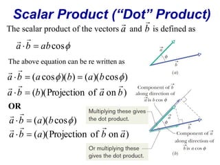
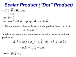
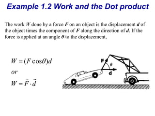
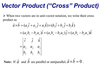
Downloaded 351 times
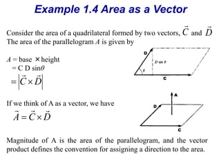
![Example 1.1 Law of Cosines
C A B
C C (A B) (A B)
2 2 2
C A B A B
2 cos
This result is generally expressed in terms of the angle φ
2 cos 2 2 2 C A B AB
[cos cos( ) cos ]](https://image.slidesharecdn.com/vkvkkchapter1-141022133915-conversion-gate01/85/Vectors-and-Kinematics-11-320.jpg)


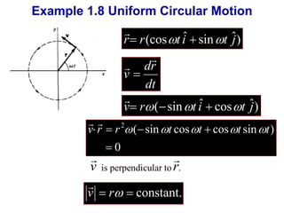
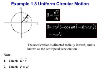
![Example 1.8 Uniform Circular Motion
Consider a particle is moving in the xy
plane according to
r r(cost iˆ sint ˆj)
[ (cos sin )] 2 2 2 1/ 2
r r t i t
r
constant
The trajectory is a circle.](https://image.slidesharecdn.com/vkvkkchapter1-141022133915-conversion-gate01/85/Vectors-and-Kinematics-31-320.jpg)
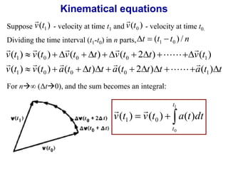
![Kinematical equations
t
1
v t v t a t dt
( ) ( ) ( ) 1 0
0
t
The above result is the same as the formal integration of
dv ( t )
a ( t )
dt
dv ( t )
a ( t )
dt
v ( t ) v ( t )
a ( t )
dt
1 0
t
1
( ) ( ) , [ ( ) intial velocity]
1 0 0 0
0
1
0
1
0
1
0
v t v a t dt v t v
t
t
t
t
t
t
t
](https://image.slidesharecdn.com/vkvkkchapter1-141022133915-conversion-gate01/85/Vectors-and-Kinematics-35-320.jpg)
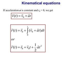
![Velocity in Polar Coordinates
d
dr
dt
dr
rr r
rr
dt
dt
v
ˆ
ˆ
( ˆ)
Recall that in cartesian coordinates -
v ( xi ˆ yj ˆ) xi ˆ yj
ˆ
d
dt
dr
dt
We know that
ˆ ˆ cos ˆ sin
r i
j
d
j
d
i
ˆ (cos ) ˆ (sin )
dt
dt
ˆ sin ˆ cos
i j
( i ˆ sin ˆ j
cos )
ˆ [ ˆ sin ˆ cos ˆ]
ˆ
i j
dr
dt
v rr r
ˆ ˆ](https://image.slidesharecdn.com/vkvkkchapter1-141022133915-conversion-gate01/85/Vectors-and-Kinematics-47-320.jpg)
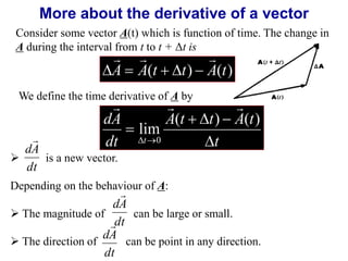
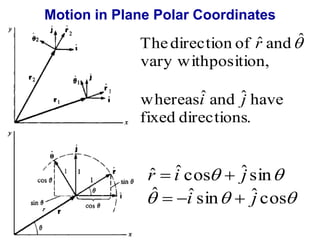
![Motion in Plane Polar Coordinates
We know that
ˆ ˆ sin ˆ cos
d
j
d
i
ˆ (sin ) ˆ (cos
)
dt
dt
ˆ cos ˆ sin
i j
(i ˆ cos ˆ j
sin )
ˆ [ ˆ cos ˆ sin ˆ]
ˆ
r i j r
d
dt
i j
r
ˆ ˆ
dr
dt
d
dt
ˆ
ˆ
](https://image.slidesharecdn.com/vkvkkchapter1-141022133915-conversion-gate01/85/Vectors-and-Kinematics-49-320.jpg)


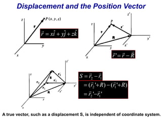
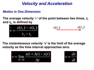
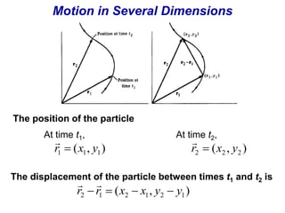
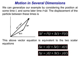
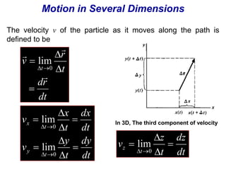
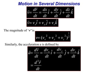
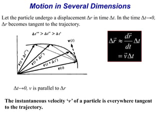
The document is a textbook chapter focused on vectors and kinematics, explaining the distinction between scalar and vector quantities. It covers vector notation, operations such as addition, subtraction, dot product, and cross product, and illustrates concepts with examples, including work done by a force and the motion of particles in one and several dimensions. Key topics include displacement, velocity, and acceleration, along with formula derivations related to mechanics.


![Motion In a Plane LNN [Lecture Note].pdf](https://cdn.slidesharecdn.com/ss_thumbnails/motioninaplanelecturenote-250429154348-b30844fd-thumbnail.jpg?width=640&height=640&fit=bounds)


