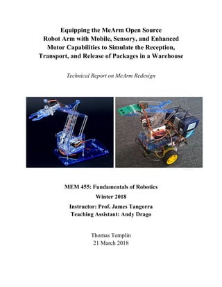
Equipping the MeArm Open Source Robot Arm with Mobile, Sensory, and Enhanced Motor Capabilities to Simulate the Reception, Transport, and Release of Packages in a Warehouse

Equipping the MeArm Open Source
Robot Arm with Mobile, Sensory, and Enhanced
Motor Capabilities to Simulate the Reception,
Transport, and Release of Packages in a Warehouse
Technical Report on MeArm Redesign
MEM 455: Fundamentals of Robotics
Winter 2018
Instructor: Prof. James Tangorra
Teaching Assistant: Andy Drago
Thomas Templin
21 March 2018

2
Proposed Useful Task
Since the 1960s, the pace of developing and implementing automated warehouse solutions has
steadily picked up. Supply-chain-automation technologies, including the deployment of
robotized warehouse systems, have strived to enhance distribution efficiency, reduce warehouse
inventory, ensure item availability, enable non-stop operation, minimize placement errors, and
reduce labor cost. Both robotic arms and mobile robots have been employed in the efficient
fulfillment of warehouse needs [1, 2].
It is proposed that the MeArm v. 1.1 be modified to simulate the distribution of items in a
warehouse. The modified MeArm implements a miniaturized and simplified version of the
following scenario: The robot serves at the receiving station of a company. It accepts packages of
uniform size, but different type, at a specific location. Depending on package type, the robot
transports a received package to one of three spatially separate storage sites in the same room of
the warehouse, one meter behind the receiving station, a distance too far to reach with a robotic
arm alone. Since the company’s operations are of a high-throughput nature and delivered goods
are being used in near real time, it is essential that the robot performs the task efficiently and
speedily.
This type of task is useful to companies that seek to automate the distribution of goods in a
warehouse. If items are to be transported to multiple storage sites that are out of reach of a
stationary arm, a hybrid mobile/arm-type robot is a feasible solution. As the MeArm is a
stationary robotic arm without any sensors, placing the MeArm on a mobile base and outfitting it
with a sensor that can detect what type of item is inside its end-effector claw requires
modifications of moderate complexity.
Needs
The robot needs to be able to fulfill a variety of needs and functions in order to successfully
complete its task. It needs to be able to move to multiple locations in the warehouse, differentiate
different types of packages, grab and hold packages securely, transport them between sites, and
release them at desired locations, satisfying logistical efficiency requirements. Primarily, the
needs relate to the robot’s performance and, secondarily, to the stakeholders’ needs. Specifically,
the robot needs to meet the following needs:
A The robot needs to be able to reach the receiving station and the warehouse storage sites
without difficulty.
B The robot needs to be able to securely grab a package (dimensions of ½  ½  ½ in3
) at a
specified (invariant) location, lift it up, retain it in its grip, and transport it to one of three

3
locations and release it. Thereafter, the robot returns to the receiving location, and the cycle
resumes.
C The robot needs to be able to differentiate three different types of packages.
D The robot needs to move at a speed that satisfies the company’s logistic requirements.
E Parts required for MeArm modification need to be available sufficiently quickly so that the
project’s overall timeframe can be met.
F The project needs to be finished by the end of the quarter.
G The project needs to remain within budget.
Specifications
Specifications translate needs into quantitative metrics that are required to satisfy the needs
associated with a device. The specifications are used to assess the success or failure of the
device’s design. The following specifications will be used to determine the adequacy and quality
of the robot’s design:
No. Need Prior-
ity
Specification Metric Value
1
2
3
A
A
B
1
1
1
Mobile base
Transport capability
Robot arm
(excluding base)
Configuration
DC-motor torque
(wheels)
Configuration
C  ℝ2
 S1
≥ 1.0 N·m
C  T2
4
5
6
7
B
B
B
B
1
1
1
1
Robot-arm material
Robot-arm lifting capability
End-effector holding capability
(Hardware + software)
tolerance
Tensile strength
Servo-motor torque
Servo-motor torque
Error (unbiased
random)
≥ 0.1 MPa
≥ 0.15 N·m
≥ 0.01 N·m
≤ 2.5 mm
8 C 1 Light sensitivity No. of reliably distin-
guishable gradations
3
9 D 2 High chassis speed Speed ≥ 40 cm/s
10 D 2 High arm speed Speed ≥ 90 deg/s
11 D 2 High gripper speed Speed ≥ 90 deg/s

4
12 E 2 Parts sourcing Time ≤ 3 business
days
13 F 1 End of Winter 2017/18 quarter Time ≤ 3/14/18
14 G 3 Total expense for modifications Purchase price ≤ $100
(ideal)
≤ $200
(if required
to satisfy
needs)
Models of MeArm v. 1.1
Degrees of Freedom
The number of the MeArm’s degrees of freedom (dof) was determined using Grübler’s formula,
where m stands for the number of degrees of freedom of a rigid body (m = 6 for spatial
mechanisms), N the number of links (including ground), J the number of joints, and fi for the
degrees of freedom provided by joint i [3]:
dof = 𝑚(𝑁 − 1 − 𝐽) + ∑ 𝑓𝑖
𝐽
𝑖=1
= 6(17 − 1 − 16) + 4 = 4.
Workspace
The approximate workspace of the MeArm’s end effector was mapped by varying the joint
angles of the servo motors of the left and right arms. The result is shown in figure 1. The legend
indicates the angular positions of the left and right servo motors. Extreme positions are indicated
by colored dots. The coordinate system is located at the top of the middle (base) servo motor.
The figure illustrates that the workspace consists of a lower portion and an upper portion with
left and right gaps in the middle.
Configurations
The arrangement of joints and linkages of the MeArm’s left and right sides are shown in figures
2 and 3, respectively. Based on the linkages’ dimensions (Li) and the joints’ orientations (θi), the
end effector’s position can be expressed as

5
Fig. 1: Approximate workspace of the MeArm’s end effector, mapped by varying the joint
angles of the servo motors of the left and right arms. The legend indicates the angular positions
of the left and right servo motors at extreme positions. The coordinate system is located at the
top of the middle (base) servo motor. The figure illustrates that the workspace consists of a lower
portion and an upper portion, with non-reachable points in the middle.
𝑥 𝑏 = 𝐿1 cos 𝜃1 + 𝐿3 cos 𝜃2 , (1)
𝑧 𝑏 = 𝐿1 sin 𝜃1 − 𝐿3 sin 𝜃2 . (2)
or
𝑥 𝑏 = 𝐿4 cos 𝜃3 + 𝐿6 cos 𝜃4 , (3)
𝑧 𝑏 = 𝐿4 sin 𝜃3 − 𝐿6 sin 𝜃4 . (4)

6
Fig. 2: Sketch of left side of MeArm.
Fig. 3: Sketch of right side of MeArm.
Forward Kinematics: Transformation Matrices and Products of Exponentials
The pose (position and orientation) of the MeArm’s linkages is described with a transformation
matrix T(θ) using the product-of-exponentials formulation. For this purpose, the MeArm was
decomposed into four parts [middle (base), left arm, right arm, and claw] describing open planar
serial chains. Figures 4–7 show the drawings of the four parts for this analysis. The dimensions
of the linkages were obtained from the CREO part files provided for the MeArm; lengths are
given in the unit of meter.
Since the MeArm’s arms contain closed loops and operate in parallel, this type of analysis is a
simplification for these parts. The simplification is valid as long as the constraints imposed by
L6
L4
L5
L4
θ4
θ3
{s}
(x1, z1)
L3
L2
L2
L1
L1
θ1
θ2
{s}
𝑧̂ 𝑠
𝑥̂ 𝑠
𝑧̂ 𝑠
𝑥̂ 𝑠
(x4, z4)

7
the parallel and closed-chain structure are taken into account. More specifically, the third joint
(θ3) of the left arm cannot assume arbitrary orientations, but is constrained by the fact that the
arm’s two vertical linkages (L2) must remain parallel. Moreover, the orientation of joint 2 (θ2) of
the right arm is determined by the orientation of joint 1 (θ1) of the left arm, which is driven by
the left servo motor.
Fig. 4: Zero position of the MeArm’s middle joint (base).
Fig. 5: Zero position of the MeArm’s left arm.
The transformation matrices T(θ) can be found by inspection from figures 4–7. They were also
calculated using individual functions from the MATLAB code provided with the textbook, as
well as by the function FKinSpace(…)[3]. The results agree. The MATLAB code for this
report is given in Appendix A.
θ1
{s}
θ4 θ3
θ2
θ1
{b} 0.115
L2 0.08
0.035
L2
L1
𝑥̂
𝑦̂
𝑧̂ 𝑠
𝑥̂ 𝑠
𝑦̂𝑠
𝑧̂ 𝑏
𝑥̂ 𝑏
𝑦̂ 𝑏

8
Fig. 6: Zero position of the MeArm’s right arm.
Fig. 7: Zero position of the MeArm’s claw (end effector).
For the middle/base, the home position is
𝑀 = [
1 0 0 0
0 1 0 0
0 0 1 0
0 0 0 1
]
and the fixed-frame screw axis
𝑆1 =
[
0
0
1
0
0
0]
.
The transformation matrix is then
𝑇(𝜃) = 𝑒[𝑆1]𝜃1 𝑀 = 𝑒
[
0 −1 0 0
1 0 0 0
0 0 0 0
0 0 0 0
]𝜃1
[
1 0 0 0
0 1 0 0
0 0 1 0
0 0 0 1
].
θ1
0.03136
L1
{b} {s}
θ3θ2
{s}
θ1
{b}
L2
0.08
L1 0.08
𝑧̂ 𝑠
𝑥̂ 𝑠
𝑦̂𝑠
𝑧̂ 𝑏
𝑦̂ 𝑏
𝑥̂ 𝑏
𝑥̂ 𝑏
𝑦̂ 𝑏
𝑥̂ 𝑠
𝑦̂𝑠

9
For the left arm, the home position is
𝑀 = [
1 0 0 0.08
0 1 0 0
0 0 1 0.08
0 0 0 1
],
and the fixed-frame screw axes are
𝑆1 =
[
0
1
0
0
0
0]
, 𝑆2 =
[
0
1
0
0
0
−0.035]
, 𝑆3 =
[
0
1
0
−0.08
0
−0.035]
, 𝑆4 =
[
0
1
0
−0.08
0
0.08 ]
.
𝑇(𝜃) = 𝑒[𝑆1]𝜃1 𝑒[𝑆2]𝜃2 𝑒[𝑆3]𝜃3 𝑒[𝑆4]𝜃4 𝑀
= 𝑒
[
0 0 1 0
0 0 0 0
−1 0 0 0
0 0 0 0
]𝜃1
𝑒
[
0 0 1 0
0 0 0 0
−1 0 0 −0.035
0 0 0 0
]𝜃2
𝑒
[
0 0 1 −0.08
0 0 0 0
−1 0 0 −0.035
0 0 0 0
]𝜃3
𝑒
[
0 0 1 −0.08
0 0 0 0
−1 0 0 0.08
0 0 0 0
]𝜃4
[
1 0 0 0.08
0 1 0 0
0 0 1 0.08
0 0 0 1
].
For the right arm, the home position is
𝑀 = [
1 0 0 0.08
0 1 0 0
0 0 1 0.08
0 0 0 1
],
and the fixed-frame screw axes are
𝑆1 =
[
0
1
0
0
0
0]
, 𝑆2 =
[
0
1
0
−0.08
0
0 ]
, 𝑆3 =
[
0
1
0
−0.08
0
0.08 ]
.
𝑇(𝜃) = 𝑒[𝑆1]𝜃1 𝑒[𝑆2]𝜃2 𝑒[𝑆3]𝜃3 𝑀
= 𝑒
[
0 0 1 0
0 0 0 0
−1 0 0 0
0 0 0 0
]𝜃1
𝑒
[
0 0 1 −0.08
0 0 0 0
−1 0 0 0
0 0 0 0
]𝜃2
𝑒
[
0 0 1 −0.08
0 0 0 0
−1 0 0 0.08
0 0 0 0
]𝜃3
[
1 0 0 0.08
0 1 0 0
0 0 1 0.08
0 0 0 1
].
For the claw (end effector), the home position is

10
𝑀 = [
1 0 0 0
0 1 0 0.03136
0 0 1 0
0 0 0 1
]
and the fixed-frame screw axis
𝑆1 =
[
0
0
1
0
0
0]
.
𝑇(𝜃) = 𝑒[𝑆1]𝜃1 𝑀 = 𝑒
[
0 −1 0 0
1 0 0 0
0 0 0 0
0 0 0 0
]𝜃1
[
1 0 0 0
0 1 0 0.03136
0 0 1 0
0 0 0 1
].
Jacobians: Twists and Wrenches
Subsequently, the space Jacobian for the left arm was derived. The Jacobian is a 64 matrix, the
columns of which correspond to the configuration-dependent screw axes. The Jacobian was
determined in two ways: using step-by-step hand calculations with the help of Maple and using
the MATLAB function JacobianSpace(…) (see Appendix A). The results agree. The space
Jacobian’s first column corresponds to the zero-position screw axis, which is S1 = (0, 1, 0, 0, 0,
0). A point on the second screw axis is given by
𝑞2 = 𝑅𝑜𝑡(𝑦̂, 𝜃1) [
−0.035
0
0
] = [
c1 0 s1
0 1 0
−s1 0 s1
] [
−0.035
0
0
] = [
−0.035c1
−0.035s1
0
].
Then, vs2 = –ωs2  q2 = (-0.035s1, 0, -0.035c1). A point on the third screw axis is given by
𝑞3 = 𝑞2 + 𝑅𝑜𝑡(𝑦̂, 𝜃1 + 𝜃2) [
0
0
0.08
] = [
−0.035c1
−0.035s1
0
] + [
c12 0 s12
0 1 0
−s12 0 s12
] [
0
0
0.08
]
= [
−0.035c1 + 0.08𝑠12
−0.035s1
0.08c12
].
Then, vs3 = –ωs3  q3 = (-0.035s1 - 0.08c12, 0, -0.035c1 + 0.08s12). A point on the third screw axis
is given by

11
𝑞4 = 𝑞3 + 𝑅𝑜𝑡(𝑦̂, 𝜃1 + 𝜃2 + 𝜃3) [
0.115
0
0
] = [
−0.035c1 + 0.08𝑠12
−0.035s1
0.08𝑐12
] + [
c123 0 s123
0 1 0
−s123 0 s123
] [
0.115
0
0
]
= [
−0.035c1 + 0.08𝑠12 + 0.115c123
−0.035s1
0.08c12 − 0.115s123
].
Then, vs4 = –ωs4  q4 = (-0.035s1 - 0.08c12 + 0.115s123, 0, -0.035c1 + 0.08s12 + 0.115c123). In these
formulae, shorthand notations for sin and cos are used. For instance, c12 = cos(θ1 + θ2) and s123 =
sin(θ1 + θ2 + θ3). Finally, based on the orientations of the screw axes (ωsi) and the calculated
linear velocities (vsi), the space Jacobian for the left arm is
𝐽𝑠(𝜃) =
[
0 0 0 0
1 1 1 1
0 0 0 0
0 −0.035s1 −0.035s1 − 0.08c12 −0.035s1 − 0.08c12 + 0.115s123
0 0 0 0
0 −0.035c1 −0.035c1 + 0.08s12 −0.035c1 + 0.08s12 + 0.115c123]
.
The space Jacobian for the right arm was calculated analogously. The result is
𝐽𝑠(𝜃) =
[
0 0 0
1 1 1
0 0 0
0 −0.08c1 −0.08c1 + 0.08s12
0 0 0
0 0.08s1 0.08s1 + 0.08c12 ]
.
The Jacobians for the middle and claw simply equal their screw axes: Js(θ) = (0, 0, 1, 0, 0, 0).
The Jacobians for the left and right arms were evaluated at arbitrary joint orientations, in order to
compare the hand calculations with the MATLAB results because the function
JacobianSpace(…) allows only numerical inputs. For the left arm, the values θ1 = 30°, θ2 = -
30°, θ3 = 30°, and θ4 = 25° were used. The result (in both Maple and MATLAB) is
𝐽𝑠(𝜃) =
[
0 0 0 0
1 1 1 1
0 0 0 0
0 −0.0175 −0.0975 −0.04
0 0 0 0
0 −0.0303 −0.0303 0.0693]
.
For the right arm, the values θ1 = 30°, θ2 = -15°, and θ3 = 60° were used, leading to the Jacobian

12
𝐽𝑠(𝜃) =
[
0 0 0
1 1 1
0 0 0
0 −0.0693 −0.0486
0 0 0
0 0.04 0.1173 ]
.
Twists (angular and linear velocities) are calculated from the Jacobian as follows:
𝒱𝑠 = 𝐽𝑠(𝜃)𝜃.̇
Assuming joint angular velocities of 𝜃̇1 = 90°/s, 𝜃̇2 = -90°/s, 𝜃̇3 = 90°/s, and 𝜃̇4 = 30°/s, the twist
for the left arm is calculated to be
𝒱𝑠 =
[
0
2.0944
0
−0.1466
0
0.0363 ]
.
Units are rad/s and m/s. Assuming joint angular velocities of 𝜃̇1 = 90°/s, 𝜃̇2 = -90°/s, 𝜃̇3 = 60°/s,
the twist for the right arm is calculated to be
𝒱𝑠 =
[
0
1.0472
0
0.058
0
0.06 ]
.
Wrenches (moments and forces) are calculated as
ℱ = 𝐽−T(𝜃)𝜏,
where τ is a column vector of joint torques. If the number of joints n ≠ 6, JT
is not invertible, and
F cannot be calculated using the above formula. In order to get around this problem, the left
Moore-Penrose pseudoinverse J†
= (JT
J)-1
JT
was used. Assuming joint torques of τ1 = 0, τ2 = 0.02
N·m, τ3 = 0.02 N·m, and τ4 = -0.04 N·m, the wrench for the left arm is
ℱ =
[
0
0.0008
0
−0.013
0
−0.5998]
.
Units are N·m and N. Assuming joint torques of τ1 = 0, τ2 = -0.03 N·m, and τ3 = - 0.07 N·m, the
wrench for the right arm is

13
ℱ =
[
0
0
0
0.1162
0
−0.5488]
.
In order to determine the required joint torques, the following formula was used:
𝜏 = 𝐽 𝑇(𝜃) ℱ.
The wrench F was determined by weighing the masses of the objects the left and right arms had
to separately support, as well as the shared masses. A mini-package/cube weighs 1.5 g.
Altogether, 50.8 g were shared, including the masses of the end effector’s servo motor and the
grayscale sensor, which had been added to fulfill the need to be able to distinguish three different
types of packages. This overall mass was equally distributed to the left and right arms. In
addition, the left arm had to support a mass of 17.3 g (self-weight) and the right arm a mass of
17.9 g (self-weight). Considering acceleration due to gravity and multiplying with a factor of 1.5
to account for joint friction, these masses amounted to left and right wrenches of F = (0 0 0 0 0 -
0.6283) and F = (0 0 0 0 0 -0.6372), respectively.
To determine the static joint torques necessary to resist the applied weights, the angular
displacements of the joints were swept across operable ranges, using nested for-loops, to
determine the Jacobian, and the maximum required torques were recorded. For the left arm, joint
angles of θ1 = [0 π], θ2 = [-π π], and θ3 = [0 π] were investigated in one-degree increments. Joint
angle 4 (θ4) is immaterial for determining the Jacobian. MATLAB computed a required
maximum torque of 0.11 N·m (see Appendix A), similar to the torque requirement given in the
specifications section (servo-motor torque ≥ 0.15 N·m), which was based on cursory analysis
using approximate loads and moment arms. For the right arm, joint angles of θ1 = [-π π] and θ2 =
[0 π] were investigated. The computed maximum torque was 0.072 N·m.
The servo’s vendor gives their torque as 1.5 kg·cm (≙ 0.147 N·m) at 5 V, which borderline
fulfills the torque requirements for the lifting capability of the robot arms (http://www.towerpro.
com.tw/product/mg90s-3/). The servo’s vendor also indicates an operating speed of 600°/s,
which certainly satisfies the speed specification, but appears unreasonably high. A detailed
velocity analysis, similar to the torque analysis, is included in Appendix A.
Inverse Kinematics
The inverse kinematics for the left arm are derived analytically from equations (1) and (2), and
for the right arm from equations (3) and (4). Since each pair of equations contains two unknowns
[(θ1 and θ2) and (θ3 and θ4), respectively], it is possible to obtain simultaneous solutions for the

14
joint angles. Symbolic solvers were run in MATLAB (see Appendix A). For the left arm, the
results are
𝜃1 =
2 atan ([2𝐿1 𝑧 𝑏 ± (−𝐿1
4
+ 2𝐿1
2
𝐿3
2
+ 2𝐿1
2
𝑥 𝑏
2
+ 2𝐿1
2
𝑧 𝑏
2
− 𝐿3
4
+ 2𝐿3
2
𝑥 𝑏
2
+ 2𝐿3
2
𝑧 𝑏
2
− 𝑥 𝑏
4
− 2𝑥 𝑏
2
𝑧 𝑏
2
− 𝑧 𝑏
4
)
1
2
] (𝐿1
2
+ 2𝐿1 𝑥 𝑏 − 𝐿3
2
+ 𝑥 𝑏
2
+ 𝑧 𝑏
2
)⁄ ) =
−2 atan ({4𝑧 𝑏 ± [−(𝑥 𝑏
2
+ 𝑧 𝑏
2
)(625𝑥 𝑏
2
+ 625𝑧 𝑏
2
− 16)]
1
2
} (25𝑥 𝑏
2
+ 4𝑥 𝑏 + 25𝑧 𝑏
2
) − 8𝑧 (25𝑥 𝑏
2
+ 4𝑥 𝑏 + 25𝑧 𝑏
2
)⁄⁄ ).
𝜃2 =
−2 atan ({2𝐿3 𝑧 𝑏 ± [(−𝐿1
2
+ 2𝐿1 𝐿3 − 𝐿3
2
+ 𝑥 𝑏
2
+ 𝑧 𝑏
2
)(𝐿1
2
+ 2𝐿1 𝐿3 + 𝐿3
2
− 𝑥 𝑏
2
− 𝑧 𝑏
2
)]
1
2
} (−𝐿1
2
+ 𝐿3
2
+ 2𝐿3 𝑥 𝑏 + 𝑥 𝑏
2
+ 𝑧 𝑏
2
)⁄ ) =
−2 atan ({4𝑧 𝑏 ± [−(𝑥 𝑏
2
+ 𝑧 𝑏
2
)(625𝑥 𝑏
2
+ 625𝑧 𝑏
2
− 16)]
1
2
} (25𝑥 𝑏
2
+ 4𝑥 𝑏 + 25𝑧 𝑏
2
)⁄ ) .
For the right arm, the results are
𝜃3 =
2 atan ([2𝐿4 𝑧 𝑏 ± (−𝐿4
4
+ 2𝐿4
2
𝐿6
2
+ 2𝐿4
2
𝑥 𝑏
2
+ 2𝐿4
2
𝑧 𝑏
2
− 𝐿6
4
+ 2𝐿6
2
𝑥 𝑏
2
+ 2𝐿6
2
𝑧 𝑏
2
− 𝑥 𝑏
4
− 2𝑥 𝑏
2
𝑧 𝑏
2
− 𝑧 𝑏
4
)
1
2
] (𝐿4
2
+ 2𝐿4 𝑥 𝑏 − 𝐿6
2
+ 𝑥 𝑏
2
+ 𝑧 𝑏
2
)⁄ ) =
−2 atan ({4𝑧 𝑏 ± [−(𝑥 𝑏
2
+ 𝑧 𝑏
2
)(625𝑥 𝑏
2
+ 625𝑧 𝑏
2
− 16)]
1
2
} (25𝑥 𝑏
2
+ 4𝑥 𝑏 + 25𝑧 𝑏
2
) − 8𝑧 (25𝑥 𝑏
2
+ 4𝑥 𝑏 + 25𝑧 𝑏
2
)⁄⁄ ).
𝜃4 =
−2 atan ({2𝐿6 𝑧 𝑏 ± [(−𝐿4
2
+ 2𝐿4 𝐿6 − 𝐿6
2
+ 𝑥 𝑏
2
+ 𝑧 𝑏
2
)(𝐿4
2
+ 2𝐿4 𝐿6 + 𝐿6
2
− 𝑥 𝑏
2
− 𝑧 𝑏
2
)]
1
2
} (−𝐿4
2
+ 𝐿6
2
+ 2𝐿6 𝑥 𝑏 + 𝑥 𝑏
2
+ 𝑧 𝑏
2
)⁄ ) =
−2 atan ({4𝑧 𝑏 ± [−(𝑥 𝑏
2
+ 𝑧 𝑏
2
)(625𝑥 𝑏
2
+ 625𝑧 𝑏
2
− 16)]
1
2
} (25𝑥 𝑏
2
+ 4𝑥 𝑏 + 25𝑧 𝑏
2
)⁄ ).
It should be noted that each equation contains two solutions (due to the ±radical). They basically
constitute elbow-up and elbow-down solutions. Since the MeArm cannot assume elbow-down
configurations, the negative-radical θ1 solution and the positive-radical θ2 solution are not
applicable.
Evaluation and Shortcomings of the MeArm v. 1.1
In its current design, the MeArm is not capable of performing the proposed task. The MeArm is
not mobile and cannot reach arbitrary locations on a planar (ℝ2
 S1
) surface (warehouse floor)
beyond the reach of its end effector. Based on the MeArm’s geometry, contrafactually assuming
that all joints can be moved independently in a serial fashion, the MeArm’s maximum forward
reach (in the x-direction) is ~19 cm. Consequently, the original MeArm is not able to reach
storage sites ≥ 1 m away from the receiving station.
Moreover, the MeArm does not have a sensor that would be able to distinguish package types.

15
The servo motors are relatively weak (minimally actuated). The servos’ vendor gives their torque
as 1.5 kg·cm (0.147 N·m) at 5 V, which borderline fulfills the torque requirements for the lifting
capability of the robot arms. The MeArm models of the previous section are approximate. For
example, the analysis was simplified by assuming serial open-loop arms. In addition, frictional
forces were not properly quantified, but roughly estimated, leading to further error in the
determination of torque requirements. Finally, dynamic torque requirements (chapter 8 of Lynch
and Park [3]) were completely neglected. During operation, the servo motors exhibited constant
jitter and unacceptable variability in orientation, making them unsuitable for the precision and
accuracy required (reproducible end-effector placement within 2.5 mm of target position).
On the other hand, the tensile strength of the linkages, the end-effector holding capability, and
the servo-motor speeds of the original MeArm are adequate.
Proposed Concept for Redesign
The MeArm is placed on a mobile base, allowing it to move freely along the warehouse floor.
The mobile base uses two DC motors, a dual H-bridge motor driver, and optical-source speed
sensors with optointerrupters and slotted encoder wheels.
Cubic packages with white, gray, and black surfaces are used, and a grayscale sensor is added to
the claw, to recognize package type based on light intensity.
The micro servo motors of the left and right arms are replaced with more powerful motors,
capable of delivering 20 kg·cm (1.96 N·m) torques. The more powerful, larger motors require
redesign of the connector arms, the motor side plates, and the corresponding motor holding
plates.
The Arduino Uno microcontroller is programmed to make the mobilized MeArm go to the
required locations (receiving station, storage sites) and grab and release packages. The weight
balance, kinematics, dynamics, power requirements, and signal-transmission electronics of the
required task are taken into account. Three sketches (robot car with speed sensor, simultaneous
control of multiple servos, and grayscale sensor) are combined into one integrated sketch. The
code for the Arduino microcontroller is given in Appendix B.
All package storage sites are 1.0 m behind the receiving station. Additionally, the storage site for
white packages is 20 cm to the right, the storage site for gray packages directly behind the
receiving station, and the storage site for black packages 20 cm to the left. The first packages of
each type are delivered directly to these locations. Subsequent packages are placed 1.5 cm to the
right of the last package of the same type. After releasing a package at a storage site, the robot

16
returns to the receiving location to accept the next package. The goal is to complete several
cycles of reception and distribution.
An approach of intertwined design, analysis, modification, and testing is adopted in an attempt to
carry out the mission with a high degree of reproducibility.
Engineering Analysis of New MeArm-based Robot
Grayscale Sensor
The analog grayscale sensor can adequately differentiate between white, gray (brown), and black
packages. Grayscale values are set to ≤ 150 for white, (150, 250] for gray, and (250 500] for
black. Ambient non-reflected light results in values higher than 500 because even black packages
reflect light from the sensor’s bright LED, so that more light reaches the sensor’s photocell than
under ambient conditions. It has to be noted though that the overall lighting conditions affect the
sensor readings, so that the sensor might need to be re-calibrated when the illumination
environment changes.
High-torque Digital Servos
The new 20 kg·cm (1.96 N·m)-torque servo motors for the left and right arms more than
adequately supply the calculated maximum torques of 0.11 N·m. The more powerful motors
eliminate the jitter and high variability of the micro servos. Ideally, new linkages made from a
stronger material would have been produced to match the higher torques of the new servos
because motor commands outside the robot arm’s range of motion might break the acrylic
linkages.
Mobile Base (diff-drive)
The primary mechanical innovation of the MeArm redesign is the mobile base. The mobile
platform greatly increases the reach of the MeArm’s end effector. The mobile base is of the diff-
drive type, with two front wheels actuated by DC motors and a caster wheel in the back [3]. This
arrangement allows the base to turn in place.
The base’s C-space is ℝ2
 S1
 S1
 S1
= ℝ2
 ϕ  θ1  θ2, where ϕ denotes the steering angle or
heading direction and θi the rotation or rolling angle of either wheel (i = 1, 2). The diff-drive
base follows Pfaffian constraints of the form 𝐴(𝑞)𝑞̇ = 0 that are not integrable, that is,

17
nonholonomic. The vector q denotes the smallest set of coordinates of the system. A bottom
view of the diff-drive is shown in figure 8 [3].
Fig. 8: Diff-drive platform used as the MeArm’s base.
Kinematic equations can now be written as
𝑥̇ = 𝑣 cos 𝜙,
𝑦̇ = 𝑣 sin 𝜙,
𝜙̇ = 𝜔,
where v denotes the platform’s forward speed and ω its rate of rotation. Then,
𝑣 =
𝑥̇
cos 𝜙
and
𝑦̇ = 𝑥̇
sin 𝜙
cos 𝜙
,
or 𝐴(𝑞)𝑞̇ = 𝑥̇ sin 𝜙 − 𝑦̇ cos 𝜙 = 0.
Let r denote the radius of a wheel disk, which rolls without slipping, and d the position vector
from the center of rotation to the point of the rotating object. Then, from v| | = rω,
𝑥̇ = 𝑟 cos 𝜙
𝜃̇ 𝑙 + 𝜃̇ 𝑟
2
,
𝑦̇ = 𝑟 sin 𝜙
𝜃̇𝑙 + 𝜃̇ 𝑟
2
.
Conversely, from ω = v⊥/d,
𝜙̇ =
1
𝑑
𝑟
𝜃̇ 𝑟 − 𝜃̇𝑙
2
.
(x, y)
d
{s}
𝑥̂ 𝑠
𝑦̂𝑠
ϕ

18
Solving simultaneously,
𝜃̇ 𝑙 =
𝑥̇ − 𝜙̇ cos 𝜙 𝑑
𝑟 cos 𝜙
=
𝑥̇
cos 𝜙
− 𝜙̇ 𝑑
𝑟
=
𝑣 − 𝜔𝑑
𝑟
,
𝜃̇ 𝑟 =
𝑥̇ + 𝜙̇ cos 𝜙 𝑑
𝑟 cos 𝜙
=
𝑥̇
cos 𝜙
+ 𝜙̇ 𝑑
𝑟
=
𝑣 + 𝜔𝑑
𝑟
.
It can be useful to control the linear velocity of a reference point P = (xP, yP) on the platform, for
instance, when a sensor (such as a camera) is located at P [3]. Employing a two-dimensional
rotation matrix, the following matrix equation holds:
[
𝑥 𝑃
𝑦 𝑃
] = [
𝑥
𝑦] + [
cos 𝜙 − sin 𝜙
sin 𝜙 cos 𝜙
] [
𝑥 𝑏
𝑦 𝑏
].
Differentiating this expression produces
[
𝑥̇ 𝑃
𝑦̇ 𝑃
] = [
𝑥̇
𝑦̇
] + 𝜙̇ [
− sin 𝜙 − cos 𝜙
cos 𝜙 − sin 𝜙
] [
𝑥 𝑏
𝑦 𝑏
].
Remembering the relationships 𝜙̇ = 𝜔, 𝑥̇ = 𝑣 cos 𝜙 , and 𝑦̇ = 𝑣 sin 𝜙, one can simultaneously
solve for v and ω to obtain
𝑣 =
𝑥 𝑏 cos 𝜙 𝑥̇ 𝑃 + 𝑦 𝑏 cos 𝜙 𝑦̇ 𝑃 − 𝑦 𝑏 sin 𝜙 𝑥̇ 𝑃 + 𝑥 𝑏 sin 𝜙 𝑦̇ 𝑃
𝑥 𝑏
=
1
𝑥 𝑏
[(𝑥 𝑟 cos 𝜙 − 𝑦𝑟 sin 𝜙)𝑥̇ 𝑃 + (𝑦𝑟 cos 𝜙 − 𝑥 𝑟 sin 𝜙)𝑦̇ 𝑃]
and
𝜔 =
cos 𝜙 𝑦̇ 𝑃 − sin 𝜙 𝑥̇ 𝑃
𝑥 𝑏
=
1
𝑥 𝑏
[− sin 𝜙 𝑥̇ 𝑃 + cos 𝜙 𝑦̇ 𝑃],
or, in matrix notation,
[
𝑣
𝜔
] = 𝐽−1(𝑞) [
𝑥̇ 𝑃
𝑦̇ 𝑃
],
where J(q) denotes the analytic Jacobian relating (v, ω) to (𝑥̇ 𝑃, 𝑦̇ 𝑃) [3].
The above analysis shows that the linear and angular velocities of the mobile platform can be
controlled to reach any point on a planar surface parameterized by the coordinates x, y, and ϕ.
Position Error
The position error for one cycle of receiving and delivering packages was determined as the
cumulative error from multiple sources. The total play/backlash between necessarily loose
connections amounted to 0.69 mm for the left arm and to 0.79 mm for the right arm.

19
Among four DC motors available to drive the base’s wheels, the two with the most similar
performances were chosen. An Arduino sketch to compare the angular speeds (rpm) of the
motors was used for this purpose [4]. Based on the distance the robot had to travel in one
reception/delivery cycle (≥ 2 m) and the average differences in the speeds of the left and right
motors, the position error due to a systematic difference in motor speeds was calculated. From
the required distance (cm), the number of steps counted by the wheels’ optical encoders and the
total number of revolutions were determined for a cycle. Comparing with the measured
difference in motor speed, the motors exhibited a directional bias of 4.63 cm per cycle, far
greater than the 2.5 mm of random error allowed by the specifications. Accordingly, without
more precise motors or a more sophisticated control system (e.g., line following), it is impossible
to correctly position the end effector over multiple cycles.
Other sources of error include random variability in motor performance (for the wheels’ DC
motors, the overall standard deviation per cycle was 3.12 cm), casting from float to int in the
integrated Arduino sketch (Appendix B), approximating π with 3.14, and slippage of the wheels
of the mobile platform.
Critical Reflection
For several decades, warehouse operations have become increasingly automated, in an effort to
improve logistical efficiency and reduce business expenditure. Companies whose receiving and
distributing operations span a rather large floor area and can be structured in a relatively
systematic way may benefit from hybrid mobile/arm-type robots equipped with sensors for the
execution of routine distribution tasks in a warehouse.
A warehouse robot needs to be able to reach the receiving station and storage sites without
difficulty, securely transport items between locations, and distinguish items by type.
Furthermore, the construction of such a robot should follow reasonable budgetary cost and time
constraints.
The current project employed a modified MeArm robot to simulate the distribution of packages
in a warehouse. In order to satisfy the needs associated with warehouse distribution tasks, a
detailed list/table of technical specifications was created. Among other things, the specification
table addresses required robot configurations, the torque and speed requirements of the various
motors used, and maximally allowed position error.
In order to acquire a better mechanical understanding of the original MeArm and to identify
necessary modifications, a detailed engineering analysis of the MeArm was performed. The
MeArm possesses four degrees of freedom, and its end effector operates in a constrained

20
workspace containing an intermediary “dead zone” along the z-axis. To simplify the
mathematical analysis, the MeArm’s left and right arms were modeled as open planar serial
chains.
Transformation matrices, product-of-exponentials formulae, and geometric space Jacobians were
derived using both software-assisted step-by-step calculations and comprehensive MATLAB
functions. The resulting equations were tested with arbitrary values, in the vicinity of anticipated
operating conditions, in order to verify the correctness of the kinematic analysis tools. In
particular, twists and wrenches were computed, using the left pseudoinverse in wrench
calculations to overcome the non-invertibility of the Jacobian.
Required torques were determined based on the total loads (package, self-weight, friction) the
left and right arms had to be able to support. The computation results show that a robot arm
needs to be able to produce at least 0.11 N·m of (static) torque. Even though the MeArm’s micro
servos are capable of torques of up to 0.15 N·m, their constant jitter and variability in
performance were deemed unacceptable.
As the simplified kinematics of the left and right arms could be expressed as two pairs of
decoupled trigonometric equations, an analytic approach was chosen for the inverse-kinematics
problem, in which joint angles are determined for pre-determined end-effector poses. The
resultant equations produced elbow-up and elbow-down solutions. The elbow-down solutions
were discarded, based on physical considerations.
The servo-motor operating speeds, the tensile strength of the linkages, and the end-effector
holding capability were determined to be satisfactory.
In order to overcome the shortcomings of the original MeArm several design modifications were
made. The MeArm was placed on a mobile base, a grayscale sensor was added to distinguish
package types, and the arms’ micro servos were replaced with more powerful servo motors
(torque rating of 1.96 N·m). An Arduino sketch was written that combined control of the motion
of the mobile base, the simultaneous control of multiple servos, and the reception and processing
of the readings of the grayscale sensor.
The grayscale sensor was capable of adequately distinguishing white, gray (brown), and black
packages. However, the sensor signal was influenced by ambient lighting conditions. The high-
torque servos eliminated the jitter and high variability observed with the micro servos.
The mobile base is of a diff-drive architecture, the kinematics of which were analyzed following
the method given in Lynch and Park [3]. A symbolic representation of the drive’s analytic

21
Jacobian was derived, relating forward speed and rate of rotation to the change in coordinates of
a point located on the platform.
Error analysis accounting for allowances between MeArm parts, systematic and random error
between the mobile base’s two DC motors, and mathematical rounding in the Arduino code
showed that end-effector positions deviated by at least 5 cm per package-reception-and-delivery
cycle, far exceeding the permitted 2.5 mm of random error per cycle.
References
[1] S. Culey, “Transformers: supply chain 3.0 and how automation will transform the rules of
the global supply chain,” The European Business Review, vol. 6, pp. 40–45, November/
December 2012.
[2] K. Azadeh and R. de Koster, “Robotized Warehouse Systems: Developments and Research
Opportunities”, SSRN, June 2017. [Online]. Available: https://papers.ssrn.com/sol3/papers.
cfm?abstract_id=2977779. [Accessed: Mar. 20, 2018].
[3] K. M. Lynch and F. C. Park, Modern Robotics: Mechanics, Planning, and Control.
Cambridge, UK: Cambridge University Press, 2017.
[4] DroneBot Workshop, “Build a Robot Car with Speed Sensors.” [Online]. Available:
https://dronebotworkshop.com/robot-car-with-speed-sensors. [Accessed: Mar. 20, 2018].
[5] S. Zolotykh, “Two Servo Motors Control through Arduino Serial.” [Online]. Available:
https://www.youtube.com/watch?v=pNI4J5EFCzA. [Accessed: Mar. 20, 2018].

Appendix A: MATLAB Code
Multi-use Variables
d2r = pi/180; % conversion from degrees to radians
r2d = 180/pi; % conversion from radians to degrees
Forward Kinematics: Transformation Matrices and Products of Exponentials
Middle/Base
M = [1 0 0 0; 0 1 0 0; 0 0 1 0; 0 0 0 1];
S1 = [0 0 1 0 0 0]';
se3mat1 = VecTose3(S1)
se3mat1 =
0 -1 0 0
1 0 0 0
0 0 0 0
0 0 0 0
% eg theta1 = 30 deg
theta1 = 30*d2r;
T = MatrixExp6((se3mat1)*theta1)*M
T =
0.8660 -0.5000 0 0
0.5000 0.8660 0 0
0 0 1.0000 0
0 0 0 1.0000
T = FKinSpace(M, S1, theta1)
T =
0.8660 -0.5000 0 0
0.5000 0.8660 0 0
0 0 1.0000 0
0 0 0 1.0000
Left arm
M = [1 0 0 .08; 0 1 0 0; 0 0 1 .08; 0 0 0 1];
S1 = [0 1 0 0 0 0]';
S2 = [0 1 0 0 0 -.035]';
S3 = [0 1 0 -.08 0 -.035]';
S4 = [0 1 0 -.08 0 .08]';
se3mat1 =
0 0 1 0
0 0 0 0
-1 0 0 0
0 0 0 0
1

se3mat2 =
0 0 1.0000 0
0 0 0 0
-1.0000 0 0 -0.0350
0 0 0 0
se3mat3 =
0 0 1.0000 -0.0800
0 0 0 0
-1.0000 0 0 -0.0350
0 0 0 0
se3mat4 =
0 0 1.0000 -0.0800
0 0 0 0
-1.0000 0 0 0.0800
0 0 0 0
% eg theta1 = 20 deg, theta2 = -20 deg, theta3 = 20 deg, theta 4 = 15 deg
theta1=20*d2r; theta2=-20*d2r; theta3=20*d2r; theta4=15*d2r;
T = MatrixExp6((se3mat1)*theta1)*MatrixExp6((se3mat2)*theta2)*...
MatrixExp6((se3mat3)*theta3)*MatrixExp6((se3mat4)*theta4)*M
T =
0.8192 0 0.5736 0.0752
0 1.0000 0 0
-0.5736 0 0.8192 0.0526
0 0 0 1.0000
T = FKinSpace(M, [S1,S2,S3,S4], [theta1 theta2 theta3 theta4]')
T =
0.8192 0 0.5736 0.0752
0 1.0000 0 0
-0.5736 0 0.8192 0.0526
0 0 0 1.0000
Right arm
M = [1 0 0 .08; 0 1 0 0; 0 0 1 .08; 0 0 0 1];
S1 = [0 1 0 0 0 0]';
S2 = [0 1 0 -.08 0 0]';
S3 = [0 1 0 -.08 0 .08]';
se3mat1 =
0 0 1 0
0 0 0 0
-1 0 0 0
0 0 0 0
2

se3mat2 =
0 0 1.0000 -0.0800
0 0 0 0
-1.0000 0 0 0
0 0 0 0
se3mat3 =
0 0 1.0000 -0.0800
0 0 0 0
-1.0000 0 0 0.0800
0 0 0 0
% eg theta1 = 20 deg, theta2 = -10 deg, theta3 = 60 deg
theta1=20*d2r; theta2=-10*d2r; theta3=60*d2r
theta3 = 1.0472
T = MatrixExp6((se3mat1)*theta1)*MatrixExp6((se3mat2)*theta2)*...
MatrixExp6((se3mat3)*theta3)*M
T =
0.3420 0 0.9397 0.1061
0 1.0000 0 0
-0.9397 0 0.3420 0.0613
0 0 0 1.0000
T = FKinSpace(M, [S1,S2,S3], [theta1 theta2 theta3]')
T =
0.3420 0 0.9397 0.1061
0 1.0000 0 0
-0.9397 0 0.3420 0.0613
0 0 0 1.0000
Claw (end effector)
M = [1 0 0 0; 0 1 0 .03136; 0 0 1 0; 0 0 0 1];
S1 = [0 0 1 0 0 0]';
se3mat1 =
0 -1 0 0
1 0 0 0
0 0 0 0
0 0 0 0
% eg theta1 = -90 deg
theta1 = -90*d2r;
T = MatrixExp6((se3mat1)*theta1)*M
T =
0.0000 1.0000 0 0.0314
3

-1.0000 0.0000 0 0.0000
0 0 1.0000 0
0 0 0 1.0000
T = FKinSpace(M, S1, theta1)
T =
0.0000 1.0000 0 0.0314
-1.0000 0.0000 0 0.0000
0 0 1.0000 0
0 0 0 1.0000
Space Jacobians
Left arm
Slist = [[0 1 0 0 0 0]', ...
[0 1 0 0 0 -.035]', ...
[0 1 0 -.08 0 -.035]', ...
[0 1 0 -.08 0 .08]'];
theta1 = 30*d2r;
theta2 = -30*d2r;
theta3 = 30*d2r;
theta4 = 25*d2r;
thetalist = [theta1 theta2 theta3 theta4]';
Jsl = JacobianSpace(Slist, thetalist)
Jsl =
0 0 0 0
1.0000 1.0000 1.0000 1.0000
0 0 0 0
0 -0.0175 -0.0975 -0.0400
0 0 0 0
0 -0.0303 -0.0303 0.0693
Right arm
Slist = [[0 1 0 0 0 0]', ...
[0 1 0 -.08 0 0]', ...
[0 1 0 -.08 0 .08]'];
S1 = [0 1 0 0 0 0]';
S2 = [0 1 0 -.08 0 0]';
theta1 = 30*d2r;
theta2 = -15*d2r;
theta3 = 60*d2r;
thetalist = [theta1 theta2 theta3]';
Jsr = JacobianSpace(Slist, thetalist)
Jsr =
0 0 0
1.0000 1.0000 1.0000
0 0 0
0 -0.0693 -0.0486
0 0 0
0 0.0400 0.1173
4

Twists
Left arm
theta1dot = 90*d2r;
theta2dot = -90*d2r;
theta3dot = 90*d2r;
theta4dot = 30*d2r;
thetadotl = [theta1dot theta2dot theta3dot theta4dot]';
Vsl = Jsl*thetadotl
Vsl =
0
2.0944
0
-0.1466
0
0.0363
Right arm
theta1dot = 90*d2r;
theta2dot = -90*d2r;
theta3dot = 60*d2r;
thetadotr = [theta1dot theta2dot theta3dot]';
Vsr = Jsr*thetadotr
Vsr =
0
1.0472
0
0.0580
0
0.0600
Wrenches
Left arm
F = [0 0 0 0 0 -(50.8/2+17.3)/1000*1.5*9.81]';
tau = Jsl'*F;
tau1 = 0;
tau2 = .02;
tau3 = .02;
tau4 = -.04;
taul = [tau1 tau2 tau3 tau4]';
F = pinv(Jsl)'*taul
F =
0.0000
0.0008
0.0000
-0.0130
0
-0.5998
5

Right arm
F = [0 0 0 0 0 -(50.8/2+17.9)/1000*1.5*9.81]';
tau = Jsr'*F;
tau1 = 0;
tau2 = -.03;
tau3 = -.07;
taur = [tau1 tau2 tau3]';
F = pinv(Jsr)'*taur
F =
-0.0000
-0.0000
0
0.1162
0
-0.5488
Determination of Robot-Arm Servo-Motor Torque Requirments
Left arm
F = [0 0 0 0 0 -(50.8/2+17.3)/1000*1.5*9.81]';
tau_l = zeros(4,1);
Slist = [[0 1 0 0 0 0]', ...
[0 1 0 0 0 -.0351]', ...
[0 1 0 -.08 0 -.0351]', ...
[0 1 0 -.08 0 .0799]'];
theta4 = 25*d2r;
for theta1 = linspace(0,pi,90)
for theta2 = linspace(-pi,pi,180)
Jsl = JacobianSpace(Slist, thetalist);
tau_l_new = Jsl'*F;
for n = 1:4
if tau_l(n) < abs(tau_l_new(n))
tau_l(n) = abs(tau_l_new(n));
end
end
end
end
end
for n = 1:4
fprintf('Max tau %d = %f N*m.n', n, tau_l(n))
end
Max tau 1 = 0.000000 N*m.
Max tau 2 = 0.022054 N*m.
Max tau 3 = 0.072319 N*m.
Max tau 4 = 0.110075 N*m.
Right arm
6

F = [0 0 0 0 0 -(50.8/2+17.9)/1000*1.5*9.81]';
tau_r = zeros(4,1);
Slist = [[0 1 0 0 0 0]', ...
[0 1 0 -.08 0 0]', ...
[0 1 0 -.08 0 .08]'];
theta3 = 60*d2r;
Jsr = JacobianSpace(Slist, thetalist);
tau_r_new = Jsr'*F;
for n = 1:3
if tau_r(n) < abs(tau_r_new(n))
tau_r(n) = abs(tau_r_new(n));
end
end
end
end
for n = 1:3
fprintf('Max tau %d = %f N*m.n', n, tau_r(n))
end
Max tau 1 = 0.000000 N*m.
Max tau 2 = 0.050971 N*m.
Max tau 3 = 0.072086 N*m.
MeArm Twist Capabilities (angular and linear velocities)
Left arm
thetadotl = [600 600 600 600]'*d2r;
Vsl = ones(6,1)*1000;
Slist = [[0 1 0 0 0 0]', ...
[0 1 0 0 0 -.0351]', ...
[0 1 0 -.08 0 -.0351]', ...
[0 1 0 -.08 0 .0799]'];
theta4 = 25*d2r;
Jsl = JacobianSpace(Slist, thetalist);
Vsl_new = Jsl*thetadotl;
for n = 1:6
if abs(Vsl_new(n)) < Vsl(n)
Vsl(n) = abs(Vsl_new(n));
end
end
end
end
end
for n = 1:3
fprintf('Min Vsl %d = %f deg/s.n', n, Vsl(n)*r2d)
7

end
Min Vsl 1 = 0.000000 deg/s.
Min Vsl 2 = 2400.000000 deg/s.
Min Vsl 3 = 0.000000 deg/s.
for n = 4:6
fprintf('Min Vsl %d = %f m.n', n, Vsl(n)*r2d)
end
Min Vsl 4 = 0.000026 m.
Min Vsl 5 = 0.000000 m.
Min Vsl 6 = 0.000031 m.
Right arm
thetadotr = [600 600 600]'*d2r;
Vsr = ones(6,1)*1000;
Slist = [[0 1 0 0 0 0]', ...
[0 1 0 -.08 0 0]', ...
[0 1 0 -.08 0 .08]'];
theta3 = 60*d2r;
Jsr = JacobianSpace(Slist, thetalist);
Vsr_new = Jsr*thetadotr;
for n = 1:6
if abs(Vsr_new(n)) < Vsr(n)
Vsr(n) = abs(Vsr_new(n));
end
end
end
end
for n = 1:3
fprintf('Min Vsr %d = %f deg/s.n', n, Vsl(n)*r2d)
end
Min Vsr 1 = 0.000000 deg/s.
Min Vsr 2 = 2400.000000 deg/s.
Min Vsr 3 = 0.000000 deg/s.
for n = 4:6
fprintf('Min Vsr %d = %f m.n', n, Vsl(n)*r2d)
end
Min Vsr 4 = 0.000026 m.
Min Vsr 5 = 0.000000 m.
Min Vsr 6 = 0.000031 m.
Inverse Kinematics
Left arm
8

Fully symbolic
syms x z L1 L3 theta1 theta2
eqns = [x == L1*cos(theta1) + L3*cos(theta2), ...
z == L1*sin(theta1) - L3*sin(theta2)];
[theta1,theta2] = solve(eqns, [theta1 theta2]);
theta1 = simplify(theta1)
theta1 =
theta2 =
Numerical (partial)
syms x z theta1 theta2
L1 = .08; L3 = .08;
theta1 =
9

theta2 =
Right arm
Fully symbolic
syms x z L4 L6 theta1 theta2
theta1 =
10

theta2 =
Numerical (partial)
syms x z theta1 theta2
L4 = .08; L6 = .08;
theta1 =
theta2 =
11

1
Appendix B: Integrated Arduino Sketch
(partially modified from [4] and [5])
#include <Servo.h>
// Constants for Interrupt Pins
// Change values if not using Arduino Uno
const byte MOTOR_A = 3; // Motor 2 Interrupt Pin - INT 1 - Right Motor
const byte MOTOR_B = 2; // Motor 1 Interrupt Pin - INT 0 - Left Motor
// Constant for steps in disk
const float stepcount = 20.00; // 20 Slots in disk, change if different
const float calibration_factor = 3.5;
// Constant for wheel diameter
const float wheeldiameter = 66.10; // Wheel diameter in mm
// Place packages 1.5 cm next to each other
float offsetWhite = 0;
float offsetGray = 0;
float offsetBlack = 0;
const float pkgDist = 1.5;
// Integers for pulse counters
volatile int counter_A = 0;
volatile int counter_B = 0;
// Motor A
int enA = 12;
int in1 = 11;
int in2 = 8;
// Motor B
int enB = 5;
int in3 = 7;
int in4 = 6;
// Digital pins for the MeArm's servo motors
int servoPinMiddle = 14;
int servoPinLeft = 15;
int servoPinRight = 16;
int servoPinClaw = 17;
// Creation of Servo objects
Servo servoMiddle;
Servo servoLeft;
Servo servoRight;
Servo servoClaw;
// Connect grayscale sensor to Analog 5
int grayScale = analogRead(5);
// Interrupt Service Routines
// Motor A pulse count ISR
void ISR_countA()
{
counter_A++; // increment Motor A counter value
}
// Motor B pulse count ISR
void ISR_countB()
{
counter_B++; // increment Motor B counter value
}
// Function to convert from centimeters to steps
int CMtoSteps(float cm) {

2
int result; // final calculation result
float circumference = (wheeldiameter*3.14)/10; // calculate wheel circumference in cm
float cm_step = circumference/stepcount; // CM per Step
float f_result = cm/cm_step; // calculate result as float
result = (int) f_result; // convert to integer (not rounded)
return result; // return result
}
// Function to convert from degrees to steps
int DEGtoSteps(float deg) {
int result; // final calculation result
float deg_step = 6; // DEG per Step
float f_result = deg/deg_step; // calculate result as float
result = (int) f_result; // convert to integer (not rounded)
return result; // End and return result
}
// Function to Move Forward
void MoveForward(int steps, int mspeed)
{
counter_A = 0; // reset counter A to zero
counter_B = 0; // reset counter B to zero
// Set Motor A forward
digitalWrite(in1, HIGH);
digitalWrite(in2, LOW);
// Set Motor B forward
// Go forward until step value is reached
while (steps > counter_A || steps > counter_B) {
if (steps > counter_A) {
analogWrite(enA, mspeed);
} else {
analogWrite(enA, 0);
}
if (steps > counter_B) {
analogWrite(enB, mspeed);
} else {
analogWrite(enB, 0);
}
}
// Stop when done
}
// Function to Move in Reverse
void MoveReverse(int steps, int mspeed)
{
// Set Motor A reverse
// Set Motor B reverse

3
// Go in reverse until step value is reached
} else {
}
} else {
}
}
// Stop when done
}
// Function to Spin Right
void SpinRight(int steps, int mspeed)
{
// Set Motor A reverse
// Set Motor B forward
// Go until step value is reached
} else {
}
} else {
}
}
// Stop when done
}
// Function to Spin Left
void SpinLeft(int steps, int mspeed)
{
// Set Motor A forward
// Set Motor B reverse

4
// Go until step value is reached
} else {
}
} else {
}
}
// Stop when done
}
void setup()
{
// Attach the Interrupts to their ISRs
attachInterrupt(digitalPinToInterrupt (MOTOR_A), ISR_countA, RISING); // Increase counter A
when speed sensor pin goes High
attachInterrupt(digitalPinToInterrupt (MOTOR_B), ISR_countB, RISING); // Increase counter B
when speed sensor pin goes High
// Attach reserved digital pins to servo motor objects
servoMiddle.attach(servoPinMiddle);
servoLeft.attach(servoPinLeft);
servoRight.attach(servoPinRight);
servoClaw.attach(servoPinClaw);
delay(3000);
}
void loop()
{
// Move robot to zero position
servoMiddle.write(90); // center base
delay(2000);
servoLeft.write(100);
delay(2000);
servoClaw.write(120); // close claw
delay(2000);
servoRight.write(100);
delay(3000);
// Move claw (end effector) to package location
servoClaw.write(20); // open claw
delay(2000);
servoLeft.write(57);
delay(2000);
servoRight.write(130);
delay(3000);
// Responding to grayscale sensor
// If white package
if (grayScale <= 250) // white
{
// Grab package
delay(2000);
servoRight.write(100); // lift arm

5
delay(2000);
// Move to warehouse location for white packages
SpinRight(DEGtoSteps(90*calibration_factor), 200); // Spin right 90 degrees at 200 speed
delay(2000);
MoveForward(CMtoSteps((20-offsetWhite)*calibration_factor), 200); // Forward (20 cm - offset)
at 200 speed
delay(2000);
delay(2000);
MoveForward(CMtoSteps(55*calibration_factor), 200); // Forward 55 cm at 200 speed
delay(2000);
// Release package
servoRight.write(125); // lower arm
delay(2000);
delay(2000);
delay(2000);
// Return to receiving station
delay(2000);
MoveForward(CMtoSteps((20-offsetWhite)*calibration_factor), 200); // Forward (20 cm - offset)
at 200 speed
delay(2000);
delay(2000);
delay(2000);
offsetWhite = offsetWhite + pkgDist;
}
// If gray package
if (grayScale > 250 && grayScale <= 320)
{
// Grab package
delay(2000);
delay(2000);
// Move to warehouse location for gray packages
SpinLeft(DEGtoSteps(90*calibration_factor), 200); // Spin left 90 degrees at 200 speed
delay(2000);
MoveForward(CMtoSteps(offsetGray*calibration_factor), 200); // Forward offset at 200 speed
delay(2000);
delay(2000);
delay(2000);
// Release package
delay(2000);
delay(2000);
delay(2000);
delay(2000);
MoveForward(CMtoSteps(offsetGray*calibration_factor), 200); // Forward offset at 200 speed
delay(2000);
delay(2000);
delay(2000);

6
offsetGray = offsetGray + pkgDist;
}
// If black package
if (grayScale > 320 && grayScale <= 360)
{
// Grab package
delay(2000);
delay(2000);
// Move to warehouse location for black packages
delay(2000);
MoveForward(CMtoSteps((20+offsetBlack)*calibration_factor), 200); // Forward offset at 200
speed
delay(2000);
delay(2000);
delay(2000);
// Release package
delay(2000);
delay(2000);
delay(2000);
delay(2000);
MoveForward(CMtoSteps((20+offsetBlack)*calibration_factor), 200); // Forward offset at 200
speed
delay(2000);
delay(2000);
delay(2000);
offsetBlack = offsetBlack + pkgDist;
}
}

Equipping the MeArm Open Source Robot Arm with Mobile, Sensory, and Enhanced Motor Capabilities to Simulate the Reception, Transport, and Release of Packages in a Warehouse

Recommended

Recommended

More Related Content

What's hot

What's hot (20)

Similar to Equipping the MeArm Open Source Robot Arm with Mobile, Sensory, and Enhanced Motor Capabilities to Simulate the Reception, Transport, and Release of Packages in a Warehouse

Similar to Equipping the MeArm Open Source Robot Arm with Mobile, Sensory, and Enhanced Motor Capabilities to Simulate the Reception, Transport, and Release of Packages in a Warehouse (20)

More from Thomas Templin

More from Thomas Templin (9)

Recently uploaded

Recently uploaded (20)

Equipping the MeArm Open Source Robot Arm with Mobile, Sensory, and Enhanced Motor Capabilities to Simulate the Reception, Transport, and Release of Packages in a Warehouse