Feature Detection in Aerial Images for Post-Disaster Needs Assessment (report)

Robotic aircraft can be rapidly deployed to capture high-resolution, low-cost aerial imagery for the purpose of post-disaster damage and needs assessment. Recently, WeRobotics, OpenAerialMap, and the World Bank captured a set of aerial images from an island state in the South Pacific, to challenge groups of qualified volunteers to develop various classifiers for baseline analysis and future damage assessment. Dr. Patrick Meier from WeRobotics made the imagery available to me, and I decided to design classifiers to detect coconut trees and asphalt/dirt roads. Four distinct object detectors (two ensembles of weak learners and two convolutional neural networks) were developed, of which two (ACF, Faster R-CNN) are based on very recently developed algorithms. Boosted ensembles of decision stumps outperformed convolutional networks in detecting coconut trees. A semantic segmentation network detected roads reasonably well, and performance might be improved by adding more training images, including synthetically generated ones.
![1
Abstract—Robotic aircraft can be rapidly deployed to capture high-resolution, low-cost aerial
imagery for the purpose of post-disaster damage and needs assessment. Recently, WeRobotics,
OpenAerialMap, and the World Bank captured a set of aerial images from an island state in the South
Pacific, to challenge groups of qualified volunteers to develop various classifiers for baseline analysis and
future damage assessment. Dr. Patrick Meier from WeRobotics made the imagery available to me, and I
decided to design classifiers to detect coconut trees and asphalt/dirt roads. Four distinct object detectors
(two ensembles of weak learners and two convolutional neural networks) were developed, of which two
(ACF, Faster R-CNN) are based on very recently developed algorithms. Boosted ensembles of decision
stumps outperformed convolutional networks in detecting coconut trees. A semantic segmentation network
detected roads reasonably well, and performance might be improved by adding more training images,
including synthetically generated ones.
I. INTRODUCTION
Robotic aircraft are employed for a variety of civil, commercial, and military applications. Observation,
surveillance, and reconnaissance tasks of robotic aircraft often include the recording, and sometimes real-time
streaming, of aerial images or videos. The ability of robotic aircraft to provide aerial imagery of a geographic
region makes them ideally suited to assess building, infrastructure, and agricultural damage in the wake of natural
disasters, as well as the needs (housing, water, food, clothing, medical care) of affected populations. Dr. Patrick
Meier is a pioneer in leveraging Big Data technology, including social media and satellite and UAV imagery, to
assess destruction and human needs caused by natural and man-made disasters. He currently serves as the
executive director and co-founder of WeRobotics, an organization that makes use of robotics, data analytics, and
machine intelligence to serve human needs in the areas of post-disaster recovery, socio-economic development,
public health, and environmental protection [2]. He also maintains an influential blog (iRevolutions.org) on these
topics.
In the iRevolutions post “Using Computer Vision to Analyze Big Data from UAVs during Disasters,” Dr.
Meier describes how volunteers use the microtasking platform MicroMappers to click on parts of videos of the
Pacific island nation Vanuatu that show building destruction caused by cyclone Pam. The clicking provides
information to the UAV pilot and humanitarian-aid teams on where to focus search-and-rescue efforts and provide
needed supplies. It also serves as ground-truth data to train visual machine-learning algorithms, to automatically
detect structural damage, without having to resort to the assistance of the clickers [3].
I became interested in using the Vanuatu clicking data for my pattern-recognition course project. After
emailing Dr. Meier and asking him about the availability of the data, he was so kind to get back to me and notify
me that the clicking data was no longer available, but that a new project was underway, in which WeRobotics,
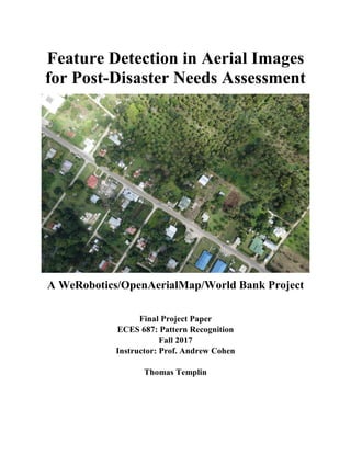
OpenAerialMap, and the World Bank was capturing aerial imagery in a South Pacific island state, to be used in a
technological challenge in which teams of volunteers develop machine-learning classifiers for the automatic
detection of various crops, coconut trees, different types of roads, and road conditions. The classifiers are to be
used for a baseline analysis for future automated damage assessment. The pictures were taken in October 2017,
and Dr. Meier generously made them available to me on November 15, 2017, prior to the public release date.
II. RELATED WORK
Aerial images can be captured by satellites or UAVs. Images from UAVs have several advantages over satellite
images: They are unaffected by atmospheric objects impeding vision, such as cloud cover or air pollution. Also,
UAV imagery is much less expensive to acquire and less affected by licensing restrictions. In addition, capturing
images using UAVs is more versatile in the sense that availability is not dependent on spatial and temporal satellite
orbit. Finally, the spatial resolution of UAV imagery is an order of magnitude higher than that of satellite imagery,
and UAV images have better color definition, important qualities for training pattern-recognition classifiers [4].
As an example, the GrassrootsMapping initiative led by Jeffrey Warren at MIT used simple UAVs, helium-filled
balloons, to chronicle the ecological devastation caused by the BP oil spill in the Gulf of Mexico in 2010, despite
the company’s attempts to restrict public access to the area [4].](data:image/gif;base64,R0lGODlhAQABAIAAAAAAAP///yH5BAEAAAAALAAAAAABAAEAAAIBRAA7)
Recommended
Recommended
More Related Content
Similar to Feature Detection in Aerial Images for Post-Disaster Needs Assessment (report)
Similar to Feature Detection in Aerial Images for Post-Disaster Needs Assessment (report) (20)
More from Thomas Templin
More from Thomas Templin (9)
Recently uploaded
Recently uploaded (20)
Feature Detection in Aerial Images for Post-Disaster Needs Assessment (report)
- 1. Feature Detection in Aerial Images for Post-Disaster Needs Assessment A WeRobotics/OpenAerialMap/World Bank Project Final Project Paper ECES 687: Pattern Recognition Fall 2017 Instructor: Prof. Andrew Cohen Thomas Templin
- 2. 1 Abstract—Robotic aircraft can be rapidly deployed to capture high-resolution, low-cost aerial imagery for the purpose of post-disaster damage and needs assessment. Recently, WeRobotics, OpenAerialMap, and the World Bank captured a set of aerial images from an island state in the South Pacific, to challenge groups of qualified volunteers to develop various classifiers for baseline analysis and future damage assessment. Dr. Patrick Meier from WeRobotics made the imagery available to me, and I decided to design classifiers to detect coconut trees and asphalt/dirt roads. Four distinct object detectors (two ensembles of weak learners and two convolutional neural networks) were developed, of which two (ACF, Faster R-CNN) are based on very recently developed algorithms. Boosted ensembles of decision stumps outperformed convolutional networks in detecting coconut trees. A semantic segmentation network detected roads reasonably well, and performance might be improved by adding more training images, including synthetically generated ones. I. INTRODUCTION Robotic aircraft are employed for a variety of civil, commercial, and military applications. Observation, surveillance, and reconnaissance tasks of robotic aircraft often include the recording, and sometimes real-time streaming, of aerial images or videos. The ability of robotic aircraft to provide aerial imagery of a geographic region makes them ideally suited to assess building, infrastructure, and agricultural damage in the wake of natural disasters, as well as the needs (housing, water, food, clothing, medical care) of affected populations. Dr. Patrick Meier is a pioneer in leveraging Big Data technology, including social media and satellite and UAV imagery, to assess destruction and human needs caused by natural and man-made disasters. He currently serves as the executive director and co-founder of WeRobotics, an organization that makes use of robotics, data analytics, and machine intelligence to serve human needs in the areas of post-disaster recovery, socio-economic development, public health, and environmental protection [2]. He also maintains an influential blog (iRevolutions.org) on these topics. In the iRevolutions post “Using Computer Vision to Analyze Big Data from UAVs during Disasters,” Dr. Meier describes how volunteers use the microtasking platform MicroMappers to click on parts of videos of the Pacific island nation Vanuatu that show building destruction caused by cyclone Pam. The clicking provides information to the UAV pilot and humanitarian-aid teams on where to focus search-and-rescue efforts and provide needed supplies. It also serves as ground-truth data to train visual machine-learning algorithms, to automatically detect structural damage, without having to resort to the assistance of the clickers [3]. I became interested in using the Vanuatu clicking data for my pattern-recognition course project. After emailing Dr. Meier and asking him about the availability of the data, he was so kind to get back to me and notify me that the clicking data was no longer available, but that a new project was underway, in which WeRobotics, OpenAerialMap, and the World Bank was capturing aerial imagery in a South Pacific island state, to be used in a technological challenge in which teams of volunteers develop machine-learning classifiers for the automatic detection of various crops, coconut trees, different types of roads, and road conditions. The classifiers are to be used for a baseline analysis for future automated damage assessment. The pictures were taken in October 2017, and Dr. Meier generously made them available to me on November 15, 2017, prior to the public release date. II. RELATED WORK Aerial images can be captured by satellites or UAVs. Images from UAVs have several advantages over satellite images: They are unaffected by atmospheric objects impeding vision, such as cloud cover or air pollution. Also, UAV imagery is much less expensive to acquire and less affected by licensing restrictions. In addition, capturing images using UAVs is more versatile in the sense that availability is not dependent on spatial and temporal satellite orbit. Finally, the spatial resolution of UAV imagery is an order of magnitude higher than that of satellite imagery, and UAV images have better color definition, important qualities for training pattern-recognition classifiers [4]. As an example, the GrassrootsMapping initiative led by Jeffrey Warren at MIT used simple UAVs, helium-filled balloons, to chronicle the ecological devastation caused by the BP oil spill in the Gulf of Mexico in 2010, despite the company’s attempts to restrict public access to the area [4].
- 3. 2 In his book “Digital Humanitarians,” Patrick Meier provides a detailed account of the development of the social media and digital technology-based humanitarian response, from crowdsourcing/searching over microtasking to machine learning and artificial intelligence [4]. Crowdsearching describes the efforts of groups of volunteers to provide information about disasters and resultant human needs using information contained in social-media messages, text messages, emails, and online photos and videos. This effort includes mapping, or geo-tagging, the locations of damage and of people in need of help. Examples include mapping efforts during the earthquake in Haiti (January 2010), Russian wildfires (summer 2010), and the civil war in Libya (starting in February 2011). The effectiveness of crowdsourcing is limited because it is rather ad-hoc and lacks effective coordination and delegation of tasks [4]. So, Patrick Meier led the development of the MicroMappers platform, a collection of microtasking apps (“clickers”), each of which processes Big Data from a certain domain, such as tweets, images, videos, and geo- tagging. The data from the individual apps are fused and integrated, to allow a more targeted and effective humanitarian response [4]. The MicroMappers video app was being deployed when volunteers catalogued the building damage in Vanuatu. MicroMappers and the Task Manager platform of the Humanitarian OpenStreetMap Team (HOT) used microtasking to perform damage and needs assessment after Typhoon Yolanda hit the Philippines in 2013. As another example, volunteers used the Tomnod microtasking platform to search for signs of Malaysia Airlines flight 370, which had gone missing in March 2014. The more recently developed “Aerial Clicker” makes tranches of images available to groups of volunteers, to search for features of interest. If five volunteers agree on the presence of a feature (e.g., damage to a certain building), the feature is considered independently verified and added to a live crisis map, together with tweets and pictures from the Tweet and Image Clickers, an illustration of grassroots-based humanitarian Big Data fusion [4]. Meanwhile, the digital humanitarian response using aerial imagery has progressed beyond crowdsearching and microtasking. The European Commission’s Joint Research Centre (JRC) in Ispra, Italy, manually tagged piles of debris in Port-au-Prince, left over from the devastating Haiti earthquake in 2010, to use as data to train a visual classifier, for the purpose of detecting rubble remaining in the capital. The classifier managed to detect almost all remaining post-earthquake debris and was used to create a heat map depicting areas of the city still riddled with rubble. The classifier’s accuracy was 92%. The Centre developed further classifiers that could spot rooftop damage and the degree of damage to a building [4]. In another project, the JRC used high-resolution satellite imagery to develop classifiers that could estimate the number of refugees, based on the number and sizes of informal shelters in a large refugee camp in Sudan. Aid organizations used the numbers to determine the amount of food and other supplies required to assist the refugees. Astoundingly, the JRC was able to use high-resolution satellite imagery to develop classifiers that could estimate the numbers of buildings (in order to track the pace of global urbanization over time), including in low-resolution Landsat images, in which buildings were not discernible with the human eye. Such post facto upsampling techniques could be used to analyze other low- resolution satellite images, such as the ones provided by the company Planet Labs, which operates a fleet of 28 micro-satellites that are capable of capturing near-real-time imagery of almost any place on Earth [4]. Based on microtasking and machine-learning experiences, a new paradigm has been emerging, in which humans and computers interact seamlessly: While humans initially annotate features in sets of images, the learning machines gradually pick up on the clues and eventually complete the feature-detection tasks automatically by themselves once enough human-generated training data has been provided. Moreover, the computer would ask for further human help if it is presented with complex cases that it had not been exposed to before [4]. In another breakthrough development, the Institute for Advanced Computer Studies at the University of Maryland has developed a computer model of poaching behavior. Using high-resolution imagery from satellites and UAVs, as well as pattern-recognition algorithms, the Institute created a model of how animals, rangers, and poachers simultaneously move through space and time. Not only can the model detect poachers, but it also predicts the type of weapon a poacher is carrying. The model is run on UAV computers in real time, providing wildlife rangers with vital timely intelligence, enhancing the chances of relatively safe intercepts and arrests [4]. For the studies presented in this paper, I chose to develop a subset of the classifiers sought by the World Bank for the South Pacific aerial-imagery data set. Classifiers were to be developed to detect (a) coconut trees and (b) asphalt and dirt roads. The development of the classifiers follows a well-defined workflow, presented in the
- 4. 3 Experimental Methods section. Four distinct object detectors (two ensembles of weak learners and two convolutional networks) were developed, and their classification performance was compared. The object detectors included two novel learning algorithms [Aggregated Channel Features (ACF) and Faster Regions with Convolutional Neural Networks (Faster R-CNN)], first introduced in MATLAB version 9.2 (R2017a). III. EXPERIMENTAL METHODS All programming tasks were performed in MATLAB (see Appendix A for code). MATLAB feature-detection capabilities were used to train various object detectors from ground-truth data, according to the following workflow [5]: • A collection of pertinent images located in a folder were loaded into the MATLAB Image Labeler app. • Features to be detected were labeled by one of two methods: A rectangular region of interest (ROI) label (“bounding box”) was placed around relevant objects (object detection), or category labels were assigned to all image pixels (semantic segmentation). • After completion of data labeling, the label locations were exported to the workspace as a table or, together with the file path of the images used, as a groundTruth object. • The exported feature labels and sets of images from which the labels had been created were used to train an ensemble of weak learners or a convolutional neural network (CNN). A. Cascade Object Detector The cascade classifier is suitable for detecting objects that are displayed at a specific orientation, so that the objects’ aspect ratio remains relatively constant. Performance decreases when the objects’ aspect ratio varies substantially because the detector is sensitive to out-of-plane rotation. The cascade classifier identifies objects in scenes by sliding windows of different sizes over the image. Thus, the classifier is capable of finding objects of variable sizes and scales, as long as variations in the aspect ratio are minor [5]. The cascade classifier uses simple image features based on mathematical operations performed on two to four rectangles spanning the space of the sliding window. As an intermediate step of these computations a so-called integral image is generated, which consists of the pixels above and to the left of a given pixel [6]. The simple features are evaluated by an ensemble of weak learners, decision stumps, i.e., one-level decision “trees,” enhanced by boosting. In boosting, samples are weighted, and a sample’s weight increases if it has been misclassified. The cascade classifier uses the AdaBoost algorithm. In AdaBoost, the sample weights wt,i are updated as follows [6-8]: 𝑤𝑡+1,𝑖 = { 𝑤𝑡,𝑖 𝑒𝑡 1 − 𝑒𝑡 if 𝑦𝑖 = 𝜙(𝑥𝑖; 𝜃𝑡) ∈ {−1,1} 𝑤𝑡,𝑖 if 𝑦𝑖 ≠ 𝜙(𝑥𝑖; 𝜃𝑡) ∈ {−1,1} , where the subscripts t and i denote the iteration and sample, respectively, et the classification error, yi the ground- truth class label, and ϕ(xi; θt) a base classifier making a binary classification decision. As shown in the formula, only the weights of correctly classified samples are updated. Updating is followed by normalization: 𝑤𝑡+1,𝑖 ← 𝑤𝑡+1,𝑖 ∑ 𝑤𝑡+1,𝑗 𝑛 𝑗=1 . The classification decision is made by weighted vote, where each classifier’s weight wt is given by 𝑤𝑡 = − log 𝑒𝑡 1 − 𝑒𝑡 . The weak-learner ensembles are arranged in stages or “cascades.” If a stage labels the current location of the sliding window as negative (i.e., the object of interest was not detected), the classification for this window is complete, and the detector moves on to the next window. A window is labeled as positive if the detector’s final stage labels the region as positive [5, 6].
- 5. 4 B. ACF Object Detector The Aggregated Channel Features (AFC) object detector computes features at finely spaced scales by means of extrapolation from nearby scales that were sampled at much coarser octave-spaced scale intervals. The detector computes channels from three families: normalized gradient magnitude, histogram of oriented gradients (six channels), and LUV color channels. Blocks of pixels are summed (“decimated”), and the lower-resolution channels are smoothed. Features are single-pixel lookups in the aggregated channels. Similar to the cascade classifier, boosting is used to train and combine decision trees/stumps over these features (pixels) to distinguish object from background using a multiscale sliding-window approach [9]. C. Faster R-CNN Regions with Convolutional Neural Networks (R-CNN) use a region proposal algorithm (e.g., Selective Search, EdgeBoxes) as a pre-processing step before running the CNN. The region proposal algorithm identifies image location in which objects are likely to be located and then processes these sites in great detail using the full power of the deep CNN. This is reminiscent of the cascade classifier, which immediately aborts processing a sliding window once it has been labeled negative (which is a frequent, but unpromising occurrence), but processes positively labeled (infrequent, but promising) regions up to the final stage. This tailored approach, as well as many other object-detection techniques, is used because of the high computational cost of the deep convolutional processing of entire images with little or no prior feature selection. Faster R-CNN integrates the region proposal mechanism into the CNN training and prediction stages and thus creates a unified region-proposal/convolutional network, which has been labeled “network with attention mechanism” [5, 10]. The CNN consists of image input, convolutional filtering, non-linear ReLU activation, fully connected output, softmax loss, and classification layers. Arbitrarily many hidden layers of adjustable width can be added. The Faster R-CNN’s loss function is given as follows [10]: 𝐿({𝑝𝑖}, {𝑡𝑖}) = 1 𝑁𝑐𝑙𝑠 ∑ 𝐿 𝑐𝑙𝑠(𝑝𝑖, 𝑝𝑖 ∗ ) 𝑖 + 𝜆 1 𝑁𝑟𝑒𝑔 ∑ 𝑝𝑖 ∗ 𝐿 𝑟𝑒𝑔(𝑡𝑖, 𝑡𝑖 ∗ ) 𝑖 . In this equation, Lcls and Ncls denote the classifier loss and normalization, respectively, Lreg and Nreg the regression loss and normalization, pi the predicted probability that a region (“anchor box”) contains the object searched for, 𝑝𝑖 ∗ the ground-truth label (0 or 1), ti a vector representing the four parameterized coordinates of the predicted bounding box, 𝑡𝑖 ∗ the vector of the ground-truth box associated with a positive anchor, and λ a hyperparameter that determines the relative weights allotted to the classification and regression losses. D. Semantic Segmentation Network Semantic segmentation also uses a CNN for visual feature detection. However, in contrast to the object detectors described above, semantic segmentation requires the assignment of a class label to every pixel of an image [11]. While object detection using a bounding box is appropriate for regular shapes that can be reasonably well enclosed by a rectangle (such as people, animals, faces, or cars), more complex geometries (buildings, streets, bridges, fields, etc.) require pixel-by-pixel labeling. In MATLAB, the semantic-segmentation CNN allows a wider range of training options than the R-CNNs described in III. C. [12]. These options specify, for example, the solver for the training network, plots showing training progress, the saving of intermediary checkpoint networks, the execution environment (e.g., CPU, GPU, parallel processing), the initial learning rate, the learning rate schedule (change over iterations), an optional regularization term, the number of epochs (full passes through the entire data set), the size of the mini batch used to evaluate the gradient of the loss function, an optional momentum term for weight/parameter updates, the shuffling of training data, and printing options for training parameters over epochs and iterations (evaluations of the gradient based on mini batches). Using stochastic gradient descent with momentum as the optimization algorithm, parameter updates are given by 𝜃𝑙+1 = 𝜃𝑙 − 𝛼𝛻𝐸(𝜃𝑙) + 𝛾(𝜃𝑙 − 𝜃𝑙−1),
- 6. 5 where θl stands for the parameter vector at epoch l, α for the learning rate, and γ for an optional momentum factor that can be added to reduce oscillations along the descent path. Weight decay, or L2 regularization, can be used to prevent overfitting: 𝐸 𝑅(𝜃) = 𝐸(𝜃) + 𝜆√𝑤 𝑇 𝑤 . The second term on the right serves as a prior on parameters to smooth out the expected value; the symbol w denotes the weight vector [12]. IV. EXPERIMENTAL RESULTS A. Cascade Object Detector and ACF Object Detector The cascade object detector was used to find coconut trees in images. The detector requires two types of image samples for classification: positive samples that display a coconut tree and negative samples that do not (Fig. 1). Sixty positive and 120 negative samples were used. The coconut trees present in the positive samples have to be enclosed in a bounding box, so that the regions of the image that are not part of the coconut tree are ignored during classifier training. The bounding boxes were drawn using the Image Labeler app, and their coordinates and dimensions (x pixel value of upper left corner, y pixel value of upper left corner, width, and height) were exported to the MATLAB workspace as a table. Fig. 1. Positive image samples containing coconut trees (left panel) and negative samples without coconut trees (right panel) used to train the cascade object detector. The positive images’ bounding boxes are not shown. The pictures were taken from the air by a UAV. Five stages (maximum number for number of images available) were used to train the cascade classifier. The false alarm rate (fraction of negative training samples incorrectly classified as positive samples) was set to 0.1 and the true positive rate (fraction of correctly classified positive training samples) to 1. In contrast to the cascade classifier, the ACF object detector requires only one set of image samples, all of which should contain at least one coconut tree. Coconut trees have to be enclosed by ROI labels. The sizes of the images should extend beyond the dimensions of the objects of interest (here, coconut trees) because the areas outside the ROIs serve as non-object or background training material for the detector (Fig. 2). Sixty images were used for training. The ACF object detector can be trained with arbitrarily many stages. For the current experiment five stages were chosen because this number was a reasonable compromise between close fit to the training data and ability to generalize to unlabeled test data and led to the detector’s best performance. Otherwise, MATLAB default settings for the classifier were used. The performance of both the cascade classifier and the ACF object detector was evaluated using two test images that were not involved in training the classifiers: a scene containing three coconut trees, as well as other vegetation and human artifacts, and a larger image containing hundreds of coconut trees. The scene with the three coconut trees is contained in and was cropped from the larger image. The number of coconut trees in the large image was determined by human count. The number amounted to 612 trees; this number served as ground truth for the large image. The performance of the classifiers is shown in in Fig. 3 and Table I. See Appendix B for the classifiers’ labeling of the large image. Obviously, there is a certain human error associated with the count of the total number of coconut trees as well as of the instances of classification error. Training and evaluation of both classifiers was fast, on the order of several minutes, when processing in parallel with four CPU cores. Fig. 2: A sample image used for training the ACF object detector, showing two coconut trees enclosed by bounding boxes and the surrounding non-object background.
- 7. 6 Fig. 3. Ability of the cascade classifier (tested on the left image) and of the ACF object detector (tested on the right image) to identify coconut trees in a scene with other plants and human-made objects. Both detectors locate the three coconut trees present. Note, however, that the cascade detector also falsely identifies a small coconut tree-like object inside the bounding box close to the image’s top left corner (left image). TABLE I PERFORMANCE METRICS FOR THE CASCADE AND ACF OBJECT DETECTORS ILLUSTRATING THEIR ABILITIES TO DETECT COCONUT TREES IN AN AERIAL PHOTOGRAPH CONTAINING HUNDREDS SUCH TREES Detector False Positive Rate (“false alarms”) False Negative Rate (“misses”) Cascade classifier 4.58% 10.29% ACF object detector 2.78% 14.71% B. Faster R-CNN Like the ACF detector, a Faster R-CNN requires bounded object images with sufficient background as input. Training of the CNN was done with the following fifteen layers: image input, 4 (convolution, ReLU), max pooling, fully connected, ReLU, fully connected, softmax, and classification output. The input size should be similar to the smallest object to be detected in the data set. The minimum horizontal size was 66 and the maximum horizontal size 151. Similarly, the minimum vertical size was 58 and the maximum vertical size 145. Consequently, an input size of (horizontal vertical rgb) of [96 96 3] was chosen. The filter size of the convolutional layers was set to 9, the number of filters to 64. Single pixels were used for zero-padding the image boundaries. The max pooling size was (w h) [5 5], with a stride of 3. Training occurred in mini-batches of size 128 and with a momentum of 0.9 (default values). Two sequences of each region proposal networks and R-CNNs were run, resulting in four consecutive networks in total. The maximum number of epochs for each network was set to 10. Learning rates were constant, 10-5 for the first RPN and R-CNN (networks 1 and 2), and 10-6 for the subsequent two networks. Small learning rates were chosen in an attempt at preventing the gradient from assuming excessively large values. As small rates slow down convergence, the max number of epochs was increased to 10, resulting in 600 iterations. Despite these efforts, classification accuracy did not converge, and the CNN experienced the “exploding gradient” problem. Variations of the above-mentioned parameters were also attempted; however, in every case, the resultant classification accuracy was either abysmal or the exploding-gradient problem was experienced (Fig. 4). The CNN could not be run many times, to experiment with more combinations of parameter settings, as a pass through the sequences of networks and layers takes longer than 48 h when training on a single CPU (in MATLAB, parallel processing is not enabled for a Faster R-CNN [5]). C. Semantic Segmentation Network Semantic segmentation was used to detect roads. All pixels of twenty images were labeled as either asphalt road, dirt road, or background (Fig. 5.; all labeled images are shown in Appendix C). The input to the semantic segmentation network includes an image datastore object, which contains the path information of the images used, (a)
- 8. 7 and a pixel label datastore object, which contains information on the pixel labels for the images in the image datastore. Fig. 5. Image showing labels for asphalt road (blue), dirt road (red), and background (yellow) (left panel). A binary mask of two asphalt roads is shown in the right panel. The semantic segmentation network consisted of the following fourteen layers: image input, 2 (convolution, ReLU, max pooling), 2 (transposed convolution, ReLU), convolution, softmax, and pixel classification. The filter size of the convolutional layers was set to 3 and the number of filters to 32. Single pixels were used for zero padding image boundaries. Both the max pool size (width and height) and the stride were set to 2. With these settings both down- and upsampling was performed. Training occurred in mini-batches of size 10, with a momentum of 0.9. The learning rate was held constant at 0.001 and the L2 regularization factor was set to 0.0005. The training data was re-shuffled at every epoch. For a maximum of 100 epochs, the training time for the network was about 10 h in parallel-processing mode (4 CPU cores). (c)Fig. 4. Inability of the Faster R-CNN to detect the object of interest and exploding-gradient problem. Using the parameter settings described in the text, the CNN was not able to identify coconut trees (a). After an initial rise, mini batch-based training accuracy would drop abruptly (b). In other cases, the gradient of the mini-batch loss would eventually become infinite (c). (b)(a)
- 9. 8 Data augmentation was used during training to provide more examples to the network in order to improve classification accuracy. For the current project, random left/right reflection and random X/Y translation of +/- 10 pixels was used for data augmentation [12]. Furthermore, class weighting was used to address class-imbalance bias, due to greatly differing pixel counts among class labels. The bias tilts predictions in favor of the dominant class. Inverse frequency weighting (class weights = inverses of class frequencies) was used to correct for the bias by increasing the weights given to under-represented classes [12] (Fig. 6; Table II). Upon completion of training, the semantic segmentation- based object detector was evaluated using a separate test image. The classifier’s ability to distinguish asphalt and dirt roads was poor. For this reason, the object-detection task was re-formulated as a binary classification problem, by combining the classes asphalt road and dirt road into a single class road, so that only the classes road and background remained. The performance of the classifier was tuned by bracketing the classification score for the combined road class. Classification scores represent the confidence in the predicted class labels. The outcome is a semantic segmentation classifier that primarily labels (asphalt and dirt) roads in red and (non-road) background in green, although parts of buildings are misclassified and, to a lesser extent, parts of vegetation (Fig. 7). Fig. 7. Performance of the semantic-segmentation object detector on a test image (left). Most road parts are labeled in red; however, there is some overlap with the classification of buildings and, to a lesser extent, of vegetation (right). V. Discussion & Conclusions The most striking finding based on the results of the studies presented is the difference in performance between the ensemble of weak learners-based object detectors and the Faster R-CNN in detecting coconut trees. While the decision stumps could be boosted to overall accuracies of greater than 90%, the convolutional network either completely failed or was not able to complete the classification task because of an exploding mini-batch gradient. This discrepancy in performance is all the more astonishing considering that the training process for the ensemble Fig. 6. Relative frequencies of the classes asphalt road, dirt road, and background in the 20 training images. TABLE II PRESENCE OF CLASS-IMBALANCE BIAS AND INVERSE-FREQUENCY RE-WEIGHTING TO CORRECT FOR IT Class Pixel Count Inverse-Frequency Class Weight Asphalt road 2.40105 44.97 Dirt road 2.85105 37.87 Background 1.027107 1.051
- 10. 9 of weak learners took at most a few minutes, whereas the training of the CNN required more than 48 h. It is possible that the CNN’s performance could be drastically improved by tuning the network using different parameter settings (types and numbers of layers, numbers of neurons per layer, filter sizes, and training options for stochastic gradient descent-based optimization). Due to time constraints, only a very limited number of variations could be attempted. Nonetheless, layers and training options were chosen based on similar classification problems reported in the literature, but the classification outcome was a complete failure. Also, CNNs are typically trained with hundreds or thousands of images, whereas the current study employed only sixty [5]. The fact still remains that, when presented with the same number of 60 training images, ensembles of very simple classifiers, that produce results very quickly and can be implemented in ten lines of code (using MATLAB toolbox functions), vastly outperformed very complex and computationally costly deep learning-based classifiers. This observation highlights another point: In pattern recognition, more complex does not translate into better, and the choice of the most appropriate classifier contains an element of art, depends on the classification task at hand, and requires the incorporation of human expert knowledge into the classification process. There are many ways to improve upon the results presented. One avenue is to employ extensive data augmentation and synthetic transformations. Random x reflections and xy translations were used to produce additional, artificially generated, images to feed to the semantic segmentation network. This approach could be applied more systematically, producing more artificial training images based on, for instance, jiggles, random crops, rotations, scale changes, and shearing [7]. Also, had more extensive testing been done, it would have been possible to present additional metrics characterizing classifier performance, such as intersection over union (IoU), boundary F-1 scores, and confusion matrices [5]. Another interesting observation was that the decisions made by the semantic segmentation network seemed to primarily rely on differences in pixel intensity and color; features based on the objects’ geometries appear to have been mostly ignored. For example, roads are mostly straight, a geometric feature the network seemed not to sufficiently capitalize on. Otherwise, many instances of misclassification of building parts and plants could have been avoided. The failure of the network to sufficiently make use of this feature may be due to the small number (20) of training images. In “Digital Humanitarians,” Patrick Meier mentions that it typically takes 72 h or longer (depending on cloud cover) to extract the features from satellite imagery required to tailor the operational aid response after a disaster. UAVs, which are becoming widely available, have the potential to narrow the time gap to 24 h. Preliminary experiments supporting rapid damage and needs assessment were carried out in the Balkans during heavy flooding in 2014 [4]. Like UAVs, pattern recognition and machine learning are technologies that bear the capacity to serve the post-disaster humanitarian aid response, as well as many other social purposes.
- 11. 10 REFERENCES [1] (6 December 2017). Unmanned aerial vehicle. Available: https://en.wikipedia.org/wiki/Unmanned_aerial_vehicle [2] (6 December 2017). WeRobotics: About Us. Available: https://werobotics.org/about-us/ [3] P. Meier, "Using Computer Vision to Analyze Big Data from UAVs during Disasters," ed, 2015. [4] P. Meier, Digital humanitarians: how big data is changing the face of humanitarian response. Crc Press, 2015. [5] Computer Vision System Toolbox: User’s Guide, Natick: The MathWorks, Inc., 2017. [Online]. Available: https://www.mathworks.com/help/pdf_doc/vision/vision_ug.pdf. Accessed on 27 November 2017. [6] P. Viola and M. Jones, "Rapid object detection using a boosted cascade of simple features," in Computer Vision and Pattern Recognition, 2001. CVPR 2001. Proceedings of the 2001 IEEE Computer Society Conference on, 2001, vol. 1, pp. I-I: IEEE. [7] I. H. Witten, E. Frank, M. A. Hall, and C. J. Pal, Data Mining: Practical machine learning tools and techniques, 4th ed. Morgan Kaufmann, 2016. [8] S. Theodoridis and K. Koutroumbas, Pattern Recognition, 4th ed. Amsterdam: Elsevier, 2009. [9] P. Dollár, R. Appel, S. Belongie, and P. Perona, "Fast feature pyramids for object detection," IEEE Transactions on Pattern Analysis and Machine Intelligence, vol. 36, no. 8, pp. 1532-1545, 2014. [10] S. Ren, K. He, R. Girshick, and J. Sun, "Faster R-CNN: Towards real-time object detection with region proposal networks," in Advances in neural information processing systems, 2015, pp. 91-99. [11] G. J. Brostow, J. Fauqueur, and R. Cipolla, "Semantic object classes in video: A high-definition ground truth database," Pattern Recognition Letters, vol. 30, no. 2, pp. 88-97, 2009. [12] M. H. Beale, M. T. Hagan, and H. B. Demuth, Neural Network Toolbox: User’s Guide, Natick: The MathWorks, Inc., 2017. [Online]. Available: https://www.mathworks.com/help/pdf_doc/nnet/nnet_ug.pdf. Accessed on 27 November 2017.
- 12. APPENDICES/SUPPLEMENTAL MATERIAL A. MATLAB Scripts (Part of the code is based on modifications from [5] and [12].) %% Cascade Object Detector (Coconut Trees) % Coconut tree images coconutTreeFolder = 'C:FinalProjectcnt_cod_expanded'; % Locations of bounding boxes load coconutTreesROIcodExpanded.mat; % Negative images negativeFolder = 'C:FinalProjectnot_cnt_cod_expanded'; % XML file in which detector parameters are stored detectorFile = 'coconutTreeDetectorExpanded.xml'; % Train detector trainCascadeObjectDetector(detectorFile, coconutTreesROIcodExpanded, ... negativeFolder, 'NumCascadeStages',5, 'FalseAlarmRate',.1, ... 'TruePositiveRate',1); %% % Use classifier to detect coconut trees detector = vision.CascadeObjectDetector(detectorFile); % Read small test image img = imread('scene_with_coconut_trees.jpg'); % Detect all coconut trees in image bbox = step(detector, img); % Demarcate detected coconut trees using bounding boxes detectedImg = insertObjectAnnotation(img,'rectangle', bbox,'coconut tree'); % Display detected coconut trees figure; imshow(detectedImg); %% % Use classifier to detect coconut trees detector = vision.CascadeObjectDetector(detectorFile); % Read large test image img = imread('DSC08896_geotag.jpg'); % Detect all coconut trees in image bbox = step(detector, img); % Demarcate detected coconut trees using bounding boxes detectedImg = insertObjectAnnotation(img,'rectangle', bbox,'coconut tree'); % Display detected coconut trees figure; imshow(detectedImg);
- 13. %% ACF Object Detector (Coconut Trees) % Load coconut tree data set load coconutTreesROIodExpanded.mat; %% Train ACF detector acfDetector = trainACFObjectDetector(coconutTreeDataset, 'NumStages',5); %% % Test detector on small test image img = imread('scene_with_coconut_trees.jpg'); [bboxes,scores] = detect(acfDetector, img); % Demarcate detected coconut trees using bounding boxes for i = 1:length(scores) annotation = sprintf('Confidence = %.1f', scores(i)); img = insertObjectAnnotation(img,'rectangle', bboxes(i,:), annotation); end figure imshow(img) %% % Test detector on large test image img = imread('DSC08896_geotag.jpg'); [bboxes,scores] = detect(acfDetector, img); % Demarcate detected coconut trees using bounding boxes for i = 1:length(scores) annotation = sprintf('Confidence = %.1f', scores(i)); img = insertObjectAnnotation(img,'rectangle', bboxes(i,:), annotation); end figure imshow(img)
- 14. %% Faster R-CNN Object Detector (Coconut Trees) % Load coconut tree data set data = load('coconutTreesROIodExpanded.mat'); coconutTreeDataset = data.coconutTreeDataset; %% Display first four rows of data set information coconutTreeDataset(1:4,:) %% Load, demarcate, and display image % Read image #10 imgNum = 10; I = imread(coconutTreeDataset.imageFilename{imgNum}); % Insert ROI labels I = insertShape(I, 'Rectangle', coconutTreeDataset.coconut_tree{imgNum}); % Resize and display image I = imresize(I, 3); figure imshow(I) %% Split data into training and test sets idx = floor(0.6 * height(coconutTreeDataset)); trainingData = coconutTreeDataset(1:idx, :); testData = coconutTreeDataset(idx:end, :); %% Create image input layer inputLayer = imageInputLayer([96 96 3]); %% Define parameters of convolutional layers % Size of local regions to which neurons connect in input filterSize = [9 9]; % Number of neurons that connect to same input region % Equals number of feature-map channels in output layer numFilters = 64; % Create middle layers middleLayers = [ convolution2dLayer(filterSize, numFilters, 'Padding', 1) reluLayer() convolution2dLayer(filterSize, numFilters, 'Padding', 1) reluLayer() % maxPooling2dLayer(5, 'Stride',3) convolution2dLayer(filterSize, numFilters, 'Padding', 1) reluLayer() convolution2dLayer(filterSize, numFilters, 'Padding', 1) reluLayer() maxPooling2dLayer(5, 'Stride',3) ]; %% Create output layers finalLayers = [ % Number of neurons in fully connected layer fullyConnectedLayer(128) % Add ReLU non-linearity reluLayer() % Last fully connected layer % Number of neurons = number of classes fullyConnectedLayer(width(coconutTreeDataset))
- 15. % Add softmax loss layer and classification layer softmaxLayer() classificationLayer() ]; %% Stack layers layers = [ inputLayer middleLayers finalLayers ] %% Training options % Region proposal network (RPN) optionsStage1 = trainingOptions('sgdm', ... 'MaxEpochs', 10, ... 'InitialLearnRate', 1e-5, ... 'VerboseFrequency', 2, ... 'CheckpointPath', tempdir); % Fast R-CNN network based on RPN optionsStage2 = trainingOptions('sgdm', ... 'MaxEpochs', 10, ... 'InitialLearnRate', 1e-5, ... 'VerboseFrequency', 2, ... 'CheckpointPath', tempdir); % Re-training of RPN using weight-sharing with Fast R-CNN optionsStage3 = trainingOptions('sgdm', ... 'MaxEpochs', 10, ... 'InitialLearnRate', 1e-6, ... 'VerboseFrequency', 2, ... 'CheckpointPath', tempdir); % Second (final) training of Fast R-CNN optionsStage4 = trainingOptions('sgdm', ... 'MaxEpochs', 10, ... 'InitialLearnRate', 1e-6, ... 'VerboseFrequency', 2, ... 'CheckpointPath', tempdir); % Combined options options = [ optionsStage1 optionsStage2 optionsStage3 optionsStage4 ]; %% Train Faster R-CNN object detector network % Set to true to train network % Set to false to load pre-trained network from disk doTrainingAndEval = true; if doTrainingAndEval % Train Faster R-CNN detector % Select box pyramid scale for multiscale object detection detector = trainFasterRCNNObjectDetector(coconutTreeDataset, layers, options, ... 'NegativeOverlapRange', [0 0.3], ... 'PositiveOverlapRange', [0.5 1], ... 'BoxPyramidScale', 1.2); else % Load pre-trained detector
- 16. detector = data.detector; end %% % Test detector on small test image I = imread('scene_with_coconut_trees.jpg'); [bboxes, scores] = detect(detector, I); % Demarcate detected coconut trees using bounding boxes I = insertObjectAnnotation(I, 'rectangle', bboxes, scores); figure imshow(I) %% % Test detector on large test image I = imread('DSC08896_geotag.jpg'); [bboxes, scores] = detect(detector, I); % Demarcate detected coconut trees using bounding boxes I = insertObjectAnnotation(I, 'rectangle', bboxes, scores); figure imshow(I)
- 17. %% Semantic Segmentation Network (Asphalt and Dirt Roads) % Load images and pixel labels imDir = 'adr_ss'; pxDir = {'C:FinalProjectPixelLabelData_24Label_1.png', ... 'C:FinalProjectPixelLabelData_24Label_2.png', ... 'C:FinalProjectPixelLabelData_24Label_3.png', ... 'C:FinalProjectPixelLabelData_24Label_4.png', ... 'C:FinalProjectPixelLabelData_24Label_5.png', ... 'C:FinalProjectPixelLabelData_24Label_6.png', ... 'C:FinalProjectPixelLabelData_24Label_7.png', ... 'C:FinalProjectPixelLabelData_24Label_8.png', ... 'C:FinalProjectPixelLabelData_24Label_9.png', ... 'C:FinalProjectPixelLabelData_24Label_10.png', ... 'C:FinalProjectPixelLabelData_24Label_11.png', ... 'C:FinalProjectPixelLabelData_24Label_12.png', ... 'C:FinalProjectPixelLabelData_24Label_13.png', ... 'C:FinalProjectPixelLabelData_24Label_14.png', ... 'C:FinalProjectPixelLabelData_24Label_15.png', ... 'C:FinalProjectPixelLabelData_24Label_16.png', ... 'C:FinalProjectPixelLabelData_24Label_17.png', ... 'C:FinalProjectPixelLabelData_24Label_18.png', ... 'C:FinalProjectPixelLabelData_24Label_19.png', ... 'C:FinalProjectPixelLabelData_24Label_20.png'}; %% Load image data using image datastore imds = imageDatastore(imDir); %% Read and display all images figure for n = 1:20 subplot(5, 4, n) I = readimage(imds,n); imshow(I) end %% % Define class names classNames = ["asphaltRoad" "dirtRoad" "background"]; % Define label ID for each class name pixelLabelID = [1 2 3]; % Create pixel label datastore pxds = pixelLabelDatastore(pxDir, classNames, pixelLabelID); %% For all images, overlay images and pixel labels figure for n = 1:20 subplot(5, 4, n) I = readimage(imds, n); C = readimage(pxds, n); B = labeloverlay(I, C); imshow(B) end %% Display image and binary mask of just asphalt roads I = readimage(imds,7); C = readimage(pxds,7); buildingMask = C == 'asphaltRoad'; figure imshowpair(I, buildingMask,'montage') %% Create image input layer inputSize = [600 900 3];
- 18. imgLayer = imageInputLayer(inputSize) %% Create downsampling network filterSize = 3; numFilters = 32; conv = convolution2dLayer(filterSize, numFilters, 'Padding',1); relu = reluLayer(); poolSize = 2; maxPoolDownsample2x = maxPooling2dLayer(poolSize, 'Stride',2); downsamplingLayers = [ conv relu maxPoolDownsample2x conv relu maxPoolDownsample2x ] %% Create upsampling network filterSize = 4; transposedConvUpsample2x = transposedConv2dLayer(4, numFilters, ... 'Stride',2, 'Cropping',1); upsamplingLayers = [ transposedConvUpsample2x relu transposedConvUpsample2x relu ] %% Create pixel classification layer numClasses = 3; conv1x1 = convolution2dLayer(1, numClasses); finalLayers = [ conv1x1 softmaxLayer() pixelClassificationLayer() ] %% Stack all layers layers = [ imgLayer downsamplingLayers upsamplingLayers finalLayers ] %% Training options for optimization algorithm (SGDM) opts = trainingOptions('sgdm', ... 'Momentum', 0.9, ... 'InitialLearnRate', 1e-3, ... 'L2Regularization', 0.0005, ... 'MaxEpochs', 100, ... 'MiniBatchSize', 10, ... 'Shuffle', 'every-epoch', ... 'ExecutionEnvironment', 'parallel', ... 'VerboseFrequency', 2, ... 'Plots', 'training-progress'); %% % Use data augmentation during training to provide more image % samples to the network to improve classification accuracy
- 19. augmenter = imageDataAugmenter('RandXReflection',true,... 'RandXTranslation', [-10 10], 'RandYTranslation',[-10 10]); trainingData = pixelLabelImageSource(imds, pxds, ... 'DataAugmentation',augmenter); %% Use inverse class frequency weighting to correct for class imbalance tbl = countEachLabel(trainingData) totalNumberOfPixels = sum(tbl.PixelCount); frequency = tbl.PixelCount / totalNumberOfPixels; classWeights = 1./frequency layers(end) = pixelClassificationLayer('ClassNames',tbl.Name, ... 'ClassWeights',classWeights); frequency = tbl.PixelCount/sum(tbl.PixelCount); figure bar(1:numel(classNames), frequency) xticks(1:numel(classNames)) xticklabels(tbl.Name) xtickangle(45) ylabel('Frequency') %% Train Semantic Segmentation Network % Set to true to train network % Set to false to load pre-trained network from disk doTraining = true; if doTraining [net,info] = trainNetwork(trainingData, layers, opts); else % Load pre-trained network data = load(pretrainedSegNet); net = data.net; end %% Read and display test image testImage = imread('DSC09699_geotag_TestImage4.jpg'); figure imshow(testImage) %% Segment test image and display results [C,score,allScores] = semanticseg(testImage, net); B = labeloverlay(testImage, C); figure imshow(B) %% Show classification scores (confidence values) figure imagesc(score) colorbar %% Bracket scores to improve classification accuracy D4 = C; for m = 1:600 for n = 1:900 if score(m,n) > .33480 && score(m,n) < .33487 D4(m,n) = 'road'; else D4(m,n) = 'background'; end end end %% Run trained network on test image and display results
- 20. E4 = labeloverlay(testImage, D4); figure imshow(E4)
- 21. B. Results for Cascade Classifier and ACF Object Detector Using Large Test Image Cascade Classifier:
- 22. ACF Detector:
- 23. C. All Images Used for Pixel Labeling (Semantic Segmentation) of Asphalt and Dirt Roads Original Images:
- 24. Labeled Images: