Downloaded 53 times

![IS Curve: Slope
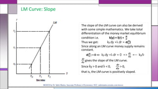
The slope of the IS curve can also be derived with some simple
mathematics. Totally differentiating the product market
equilibrium condition i.e. y = c(y-t(y)) + i(r) + g
=> dy = cy (dy – ty dy) + ir dr + g
Assuming g constant i.e. dg = 0, we get [dy – cy (1 – ty)dy] = ir dr
=> [1 –cy (1 - ty)] dy = ir dr
=>
𝒅𝒓
𝒅𝒚
=
[1 –cy (1 −ty)]
ir
Since we know that [1 –cy (1 - ty)] > 0, and ir < 0, it is clear
that
𝒅𝒓
𝒅𝒚
< 0. This shows that the slope the IS curve in Figure is
negative.
MOOCS by Dr. Subir Maitra, Associate Professor of Economics, HCC, subirmaitra.wixsite.com/moocs](https://image.slidesharecdn.com/is-lmmodel2-180605131358/85/IS-LM-Model-2-9-320.jpg)

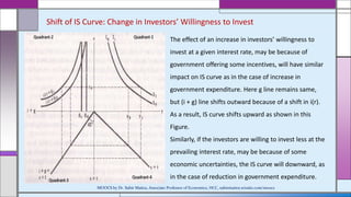
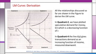
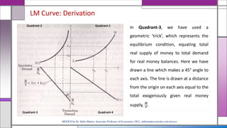
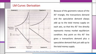
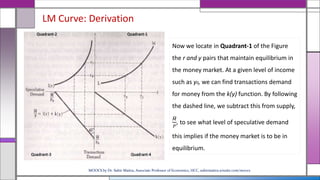
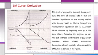
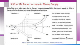
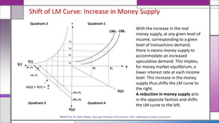
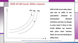


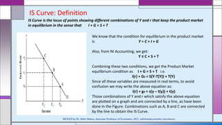
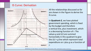
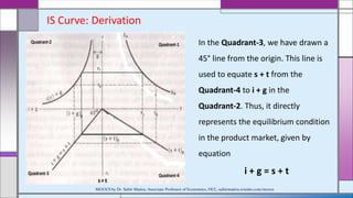
This document provides an overview of the IS-LM model and how it can be used to analyze macroeconomic equilibrium. It discusses the derivation of the IS and LM curves from the equilibrium conditions of the goods market and money market. The IS curve represents combinations of interest rates and income that balance investment, savings, taxes and government spending. The LM curve represents combinations of interest rates and income that equate the demand and supply of money. The document examines how shifts in factors like money supply, government spending, taxes and savings preferences cause the IS and LM curves to shift. This allows analyzing their impact on equilibrium income and interest rates.