Downloaded 79 times


![Julia code
a = [1, 2, 3, 4, 5]
function square(x)
return x^2
end
for x in a
println(square(x))
end
11](https://image.slidesharecdn.com/20180811coscup-180811040007/85/COSCUP-Introduction-to-Julia-11-320.jpg)


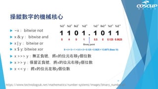


![電腦怎麼出拳
rand(): 隨機0~1
rand([]): 從裡面選一個出來
y = rand([1, 2, 3])
59](https://image.slidesharecdn.com/20180811coscup-180811040007/85/COSCUP-Introduction-to-Julia-59-320.jpg)


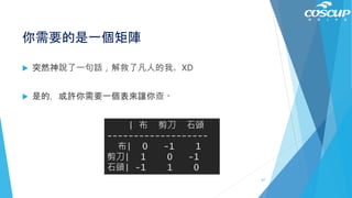
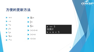
![介紹Array
homogenous
start from 1
mutable
[ ]2 3 5
A = [2, 3, 5]
A[2] # 3
68](https://image.slidesharecdn.com/20180811coscup-180811040007/85/COSCUP-Introduction-to-Julia-68-320.jpg)
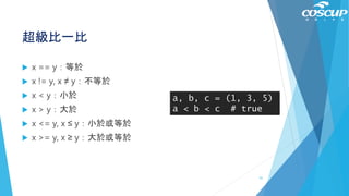
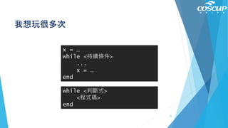
![多維陣列
A = [0, -1, 1;
1, 0, -1;
-1, 1, 0]
A[1, 2]
69](https://image.slidesharecdn.com/20180811coscup-180811040007/85/COSCUP-Introduction-to-Julia-69-320.jpg)

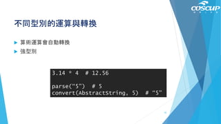
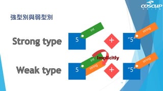
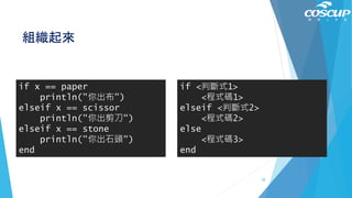
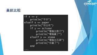
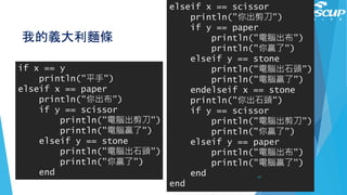
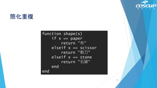
![簡化完畢
稱為重構
refactoring
x_shape = shape(x)
y_shape = shape(y)
println("你出" * x_shape)
println("電腦出" * y_shape)
win_or_lose = A[x, y]
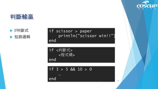
if win_or_lose == 0
println("平手")
elseif win_or_lose == 1
println("你贏了")
else
println("電腦贏了")
end
71](https://image.slidesharecdn.com/20180811coscup-180811040007/85/COSCUP-Introduction-to-Julia-71-320.jpg)

![Array搭配for loop
strings = ["foo","bar","baz"]
for s in strings
println(s)
end
76](https://image.slidesharecdn.com/20180811coscup-180811040007/85/COSCUP-Introduction-to-Julia-76-320.jpg)
![Comprehension
[x for x = 1:3]
[x for x = 1:20 if x % 2 == 0]
["$x * $y = $(x*y)" for x=1:9, y=1:9]
[1, 2, 3]
[2, 4, 6, 8, 10, 12, 14, 16, 18, 20]
[“1 * 1 = 1“, “1 * 2 = 2“, “1 * 3 = 3“ ...]
78](https://image.slidesharecdn.com/20180811coscup-180811040007/85/COSCUP-Introduction-to-Julia-78-320.jpg)
![Tuple
Immutable
tup = (1, 2, 3)
tup[1] # 1
tup[1:2] # (1, 2)
(a, b, c) = (1, 2, 3)
79](https://image.slidesharecdn.com/20180811coscup-180811040007/85/COSCUP-Introduction-to-Julia-79-320.jpg)
![Set
Mutable
filled = Set([1, 2, 2, 3, 4])
push!(filled, 5)
intersect(filled, other)
union(filled, other)
setdiff(Set([1, 2, 3, 4]), Set([2, 3, 5]))
Set([i for i=1:10])
80](https://image.slidesharecdn.com/20180811coscup-180811040007/85/COSCUP-Introduction-to-Julia-80-320.jpg)
![Dict
Mutable
filled = Dict("one"=> 1, "two"=> 2, "three"=> 3)
keys(filled)
values(filled)
Dict(x=> i for (i, x) in enumerate(["one", "two",
"three", "four"]))
81](https://image.slidesharecdn.com/20180811coscup-180811040007/85/COSCUP-Introduction-to-Julia-81-320.jpg)


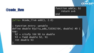
![@code_native
julia> @code_native add(1, 2)
.text
Filename: REPL[2]
pushq %rbp
movq %rsp, %rbp
Source line: 2
leaq (%rcx,%rdx), %rax
popq %rbp
retq
nopw (%rax,%rax)
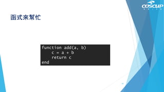
function add(a, b)
return a+b
end
88](https://image.slidesharecdn.com/20180811coscup-180811040007/85/COSCUP-Introduction-to-Julia-88-320.jpg)

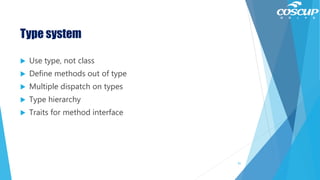


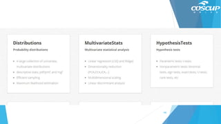


![DataFrames.jl
julia> using DataFrames
julia> dt = DataFrame(A = 1:4, B = ["M", "F", "F", "M"])
4×2 DataFrames.DataFrame
│ Row │ A │ B │
├─────┼───┼───┤
│ 1 │ 1 │ M │
│ 2 │ 2 │ F │
│ 3 │ 3 │ F │
│ 4 │ 4 │ M │
103](https://image.slidesharecdn.com/20180811coscup-180811040007/85/COSCUP-Introduction-to-Julia-103-320.jpg)
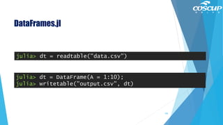
![DataFrames.jl
julia> dt[:A]
4-element NullableArrays.NullableArray{Int64,1}:
1
2
3
4
julia> dt[2, :A]
Nullable{Int64}(2)
104](https://image.slidesharecdn.com/20180811coscup-180811040007/85/COSCUP-Introduction-to-Julia-104-320.jpg)
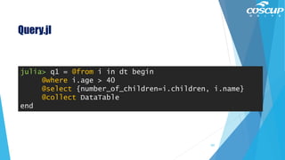
![DataFrames.jl
julia> names = DataFrame(ID = [1, 2], Name = ["John
Doe", "Jane Doe"])
julia> jobs = DataFrame(ID = [1, 2], Job = ["Lawyer",
"Doctor"])
julia> full = join(names, jobs, on = :ID)
2×3 DataFrames.DataFrame
│ Row │ ID │ Name │ Job │
├─────┼────┼──────────┼────────┤
│ 1 │ 1 │ John Doe │ Lawyer │
│ 2 │ 2 │ Jane Doe │ Doctor │ 106](https://image.slidesharecdn.com/20180811coscup-180811040007/85/COSCUP-Introduction-to-Julia-106-320.jpg)
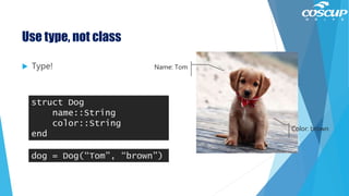
![StatsBase.jl
Mean Functions
mean(x, w)
geomean(x)
harmmean(x)
Scalar Statistics
var(x, wv[; mean=...])
std(x, wv[; mean=...])
mean_and_var(x[, wv][, dim])
mean_and_std(x[, wv][, dim])
zscore(X, μ, σ)
entropy(p)
crossentropy(p, q)
kldivergence(p, q)
percentile(x, p)
nquantile(x, n)
quantile(x)
median(x, w)
mode(x)
108](https://image.slidesharecdn.com/20180811coscup-180811040007/85/COSCUP-Introduction-to-Julia-108-320.jpg)
![StatsBase.jl
Sampling from Population
sample(a)
Correlation Analysis of Signals
autocov(x, lags[; demean=true])
autocor(x, lags[; demean=true])
corspearman(x, y)
corkendall(x, y)
109](https://image.slidesharecdn.com/20180811coscup-180811040007/85/COSCUP-Introduction-to-Julia-109-320.jpg)
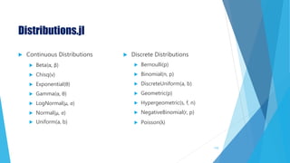
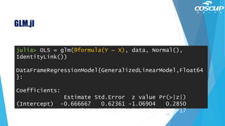
![GLM.jl
111
julia> data = DataFrame(X=[1,2,3], Y=[2,4,7])
3x2 DataFrame
|-------|---|---|
| Row # | X | Y |
| 1 | 1 | 2 |
| 2 | 2 | 4 |
| 3 | 3 | 7 |](https://image.slidesharecdn.com/20180811coscup-180811040007/85/COSCUP-Introduction-to-Julia-111-320.jpg)
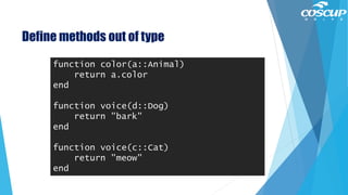
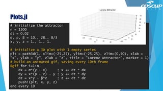
![GLM.jl
113
julia> newX = DataFrame(X=[2,3,4]);
julia> predict(OLS, newX, :confint)
3×3 Array{Float64,2}:
4.33333 1.33845 7.32821
6.83333 2.09801 11.5687
9.33333 1.40962 17.257
# The columns of the matrix are prediction, 95% lower
and upper confidence bounds](https://image.slidesharecdn.com/20180811coscup-180811040007/85/COSCUP-Introduction-to-Julia-113-320.jpg)


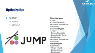


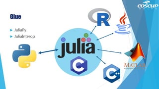


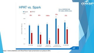
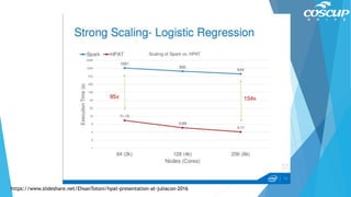
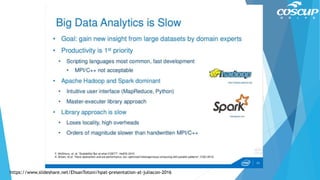


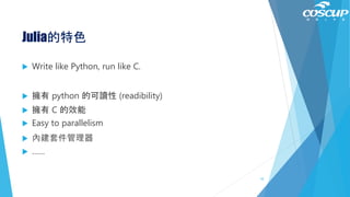
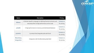
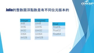
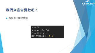
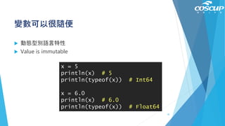
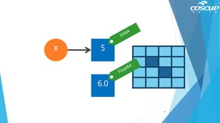
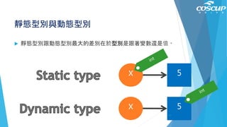
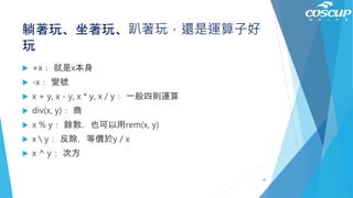
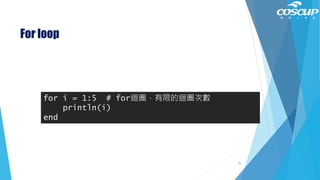
This document provides an introduction to the Julia programming language. It discusses key features of Julia such as writing code that is readable like Python but runs as fast as C. Examples are given showing Julia's dynamic typing, numeric types, operators, control flow statements like if/else and while loops, and arrays. The document ends with a rock-paper-scissors game example that demonstrates functions, conditionals, and refactoring code for simplicity.


![[COSCUP 2023] 我的Julia軟體架構演進之旅](https://cdn.slidesharecdn.com/ss_thumbnails/slides-230807142223-9909fa32-thumbnail.jpg?width=640&height=640&fit=bounds)


