Downloaded 12 times


![Julia code
a = [1, 2, 3, 4, 5]
function square(x)
return x^2
end
for x in a
println(square(x))
end
10](https://image.slidesharecdn.com/20180610introductiontojulia-180610151833/85/Introduction-to-Julia-10-320.jpg)


![Array 搭配 for loop
strings = ["foo","bar","baz"]
for s in strings
println(s)
end
33](https://image.slidesharecdn.com/20180610introductiontojulia-180610151833/85/Introduction-to-Julia-33-320.jpg)
![Rand()
rand(): 隨機0~1
rand([]): 從裡面選一個出來
y = rand([1, 2, 3])
34](https://image.slidesharecdn.com/20180610introductiontojulia-180610151833/85/Introduction-to-Julia-34-320.jpg)
![Array
homogenous
start from 1
mutable
[ ]2 3 5
A = [2, 3, 5]
A[2] # 3
35](https://image.slidesharecdn.com/20180610introductiontojulia-180610151833/85/Introduction-to-Julia-35-320.jpg)
![多維陣列
A = [0 -1 1;
1 0 -1;
-1 1 0]
A[1, 2]
36](https://image.slidesharecdn.com/20180610introductiontojulia-180610151833/85/Introduction-to-Julia-36-320.jpg)
![Comprehension
[x for x = 1:3]
[x for x = 1:20 if x % 2 == 0]
["$x * $y = $(x*y)" for x=1:9, y=1:9]
[1, 2, 3]
[2, 4, 6, 8, 10, 12, 14, 16, 18, 20]
[“1 * 1 = 1“, “1 * 2 = 2“, “1 * 3 = 3“ ...]
40](https://image.slidesharecdn.com/20180610introductiontojulia-180610151833/85/Introduction-to-Julia-40-320.jpg)
![Tuple
Immutable
tup = (1, 2, 3)
tup[1] # 1
tup[1:2] # (1, 2)
(a, b, c) = (1, 2, 3)
41](https://image.slidesharecdn.com/20180610introductiontojulia-180610151833/85/Introduction-to-Julia-41-320.jpg)
![Set
Mutable
filled = Set([1, 2, 2, 3, 4])
push!(filled, 5)
intersect(filled, other)
union(filled, other)
setdiff(Set([1, 2, 3, 4]), Set([2, 3, 5]))
Set([i for i=1:10])
42](https://image.slidesharecdn.com/20180610introductiontojulia-180610151833/85/Introduction-to-Julia-42-320.jpg)
![Dict
Mutable
filled = Dict("one"=> 1, "two"=> 2, "three"=> 3)
keys(filled)
values(filled)
Dict(x=> i for (i, x) in enumerate(["one", "two",
"three", "four"]))
43](https://image.slidesharecdn.com/20180610introductiontojulia-180610151833/85/Introduction-to-Julia-43-320.jpg)


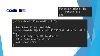
![@code_native
julia> @code_native add(1, 2)
.text
Filename: REPL[2]
pushq %rbp
movq %rsp, %rbp
Source line: 2
leaq (%rcx,%rdx), %rax
popq %rbp
retq
nopw (%rax,%rax)
function add(a, b)
return a+b
end
51](https://image.slidesharecdn.com/20180610introductiontojulia-180610151833/85/Introduction-to-Julia-51-320.jpg)


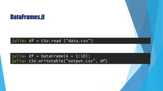
![DataFrames.jl
julia> using DataFrames
julia> df = DataFrame(A = 1:4, B = ["M", "F", "F", "M"])
4×2 DataFrames.DataFrame
│ Row │ A │ B │
├─────┼───┼───┤
│ 1 │ 1 │ M │
│ 2 │ 2 │ F │
│ 3 │ 3 │ F │
│ 4 │ 4 │ M │
59](https://image.slidesharecdn.com/20180610introductiontojulia-180610151833/85/Introduction-to-Julia-59-320.jpg)
![DataFrames.jl
julia> df[:A]
4-element NullableArrays.NullableArray{Int64,1}:
1
2
3
4
julia> df[2, :A]
Nullable{Int64}(2)
60](https://image.slidesharecdn.com/20180610introductiontojulia-180610151833/85/Introduction-to-Julia-60-320.jpg)
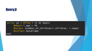
![DataFrames.jl
julia> names = DataFrame(ID = [1, 2], Name = ["John
Doe", "Jane Doe"])
julia> jobs = DataFrame(ID = [1, 2], Job = ["Lawyer",
"Doctor"])
julia> full = join(names, jobs, on = :ID)
2×3 DataFrames.DataFrame
│ Row │ ID │ Name │ Job │
├─────┼────┼──────────┼────────┤
│ 1 │ 1 │ John Doe │ Lawyer │
│ 2 │ 2 │ Jane Doe │ Doctor │ 62](https://image.slidesharecdn.com/20180610introductiontojulia-180610151833/85/Introduction-to-Julia-62-320.jpg)
![StatsBase.jl
Mean Functions
mean(x, w)
geomean(x)
harmmean(x)
Scalar Statistics
var(x, wv[; mean=...])
std(x, wv[; mean=...])
mean_and_var(x[, wv][, dim])
mean_and_std(x[, wv][, dim])
zscore(X, μ, σ)
entropy(p)
crossentropy(p, q)
kldivergence(p, q)
percentile(x, p)
nquantile(x, n)
quantile(x)
median(x, w)
mode(x)
64](https://image.slidesharecdn.com/20180610introductiontojulia-180610151833/85/Introduction-to-Julia-64-320.jpg)
![StatsBase.jl
Sampling from Population
sample(a)
Correlation Analysis of Signals
autocov(x, lags[; demean=true])
autocor(x, lags[; demean=true])
corspearman(x, y)
corkendall(x, y)
65](https://image.slidesharecdn.com/20180610introductiontojulia-180610151833/85/Introduction-to-Julia-65-320.jpg)

![GLM.jl
67
julia> data = DataFrame(X=[1,2,3], Y=[2,4,7])
3x2 DataFrame
|-------|---|---|
| Row # | X | Y |
| 1 | 1 | 2 |
| 2 | 2 | 4 |
| 3 | 3 | 7 |](https://image.slidesharecdn.com/20180610introductiontojulia-180610151833/85/Introduction-to-Julia-67-320.jpg)
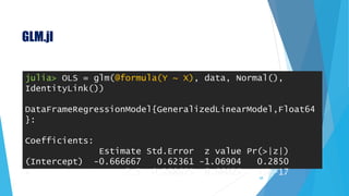
![GLM.jl
69
julia> newX = DataFrame(X=[2,3,4]);
julia> predict(OLS, newX, :confint)
3×3 Array{Float64,2}:
4.33333 1.33845 7.32821
6.83333 2.09801 11.5687
9.33333 1.40962 17.257
# The columns of the matrix are prediction, 95% lower
and upper confidence bounds](https://image.slidesharecdn.com/20180610introductiontojulia-180610151833/85/Introduction-to-Julia-69-320.jpg)


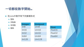
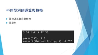
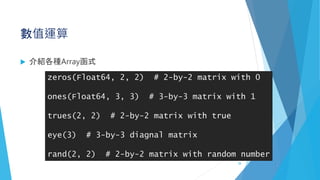
This document introduces Julia and provides an overview of its key features. It begins with introductions and background on why Julia was created. It then covers basic Julia concepts like variables, arithmetic operators, control flow, arrays, functions, and parallelization capabilities. The document also discusses Julia's built-in package ecosystem and provides examples of packages like DataFrames. It aims to provide attendees with foundational knowledge of the Julia programming language.


![[系列活動] 手把手的深度學實務](https://cdn.slidesharecdn.com/ss_thumbnails/slidedlfinal1216-171213041058-thumbnail.jpg?width=640&height=640&fit=bounds)
![[系列活動] 手把手的深度學習實務](https://cdn.slidesharecdn.com/ss_thumbnails/slidesharestepbystepdl-161213072731-thumbnail.jpg?width=640&height=640&fit=bounds)

![[系列活動] Data exploration with modern R](https://cdn.slidesharecdn.com/ss_thumbnails/dataexplorationwithmodernr1221-161219044516-thumbnail.jpg?width=640&height=640&fit=bounds)


![[COSCUP 2023] 我的Julia軟體架構演進之旅](https://cdn.slidesharecdn.com/ss_thumbnails/slides-230807142223-9909fa32-thumbnail.jpg?width=640&height=640&fit=bounds)


![Getting Started with Apache Spark: Big Data Made Simple [Free Meetup]](https://cdn.slidesharecdn.com/ss_thumbnails/apachesparkgettingstarted-260203175547-8361bcc3-thumbnail.jpg?width=640&height=640&fit=bounds)


