SlideShare a Scribd company logo
1 of 11
Download to read offline
SM/CU/MCOM/FIRST YEAR/MEBE/MOD-I/2017-18 MOOCS: subirmaitra.wixsite.com/moocs 1
2.1 Introduction:
If we plot the values of GDP of any country over a period of say, fifty years, we will find a
periodic fluctuation around some trend line. These systematic fluctuations in the level of aggregate
economic activity is known as business cycles consisting of booms or expansions and recessions or
contraction. The long run model of the economy cannot explain recession or boom when the economy
deviates from its long run path.
GDP
Time
Figure: 1
To understand what kind of forces is responsible for these fluctuations in real output relative
to trend, we develop ‘Keynesian Model’. The cornerstone of this model is the mutual interaction
between output and spending: spending determines output and income, and at the same time, output
and income also determine spending.
We shall first develop a very simple model of income determination known as Simple
Keynesian Model. This most important assumption of this model is that prices are constant. In the
short run, firms stand ready to supply whatever output their customers want at the given prices. Thus,
demand becomes the ruling force in this model. If demand is strong, real GDP exceeds potential. In
recession, when demand is weak, real GDP drops below potential.
2.2 Simple Keynesian Model:
The Simple Keynesian Model is a static model of the economy which helps us to determine
equilibrium real national income based on ‘effective demand’ principle.
Equilibrium Income: Cases of Open and Closed Economies, Multiplier theory-
Keynesian Approach
Lecture-1
SM/CU/MCOM/FIRST YEAR/MEBE/MOD-I/2017-18 MOOCS: subirmaitra.wixsite.com/moocs 2
2.2.1 Assumptions:
(i) One-sector model: The SKM is a one-sector model which includes only the goods
market.
(ii) Absence of monetary sector: There is no monetary sector in the SKM.
(iii) Static model: The SKM is a static model. The model solves for static equilibrium
level of real output, which is the value of real output that has no tendency to change
once it has been established.
(iv) Closed economy with or without Government: The SKM assumes a closed
economy (i.e. without foreign trade) with or without Government.
(v) Constant prices: In stark contrast to the quantity theory model, the SKM assumes
an exogenously fixed price level.
(vi) Short-run model: The model is a short-run model and determines the value of real
national output for a particular period of time, such as a year.
(vii) Fixed stock of capital and labour: The model assumes that both the stock of
capital and the labour force, which when fully utilised determine the maximum level
of real output the economy can produce, are constant.
(viii) Profit maximization: An underlying behavioural assumption of the model is that
firms act as profit maximisers. If demand for their output exceeds supply, firms
increase production, providing there are spare resources put to work. Conversely if
supply exceeds demand, firms reduce output.
(ix) Effective demand principle: The SKM is based on Keynesian ‘effective demand
principle’. According to this principle, since commodities are necessarily produced
for a market, the size of the market must regulate the level of commodity production.
Put differently, effective demand refers to that level of the value of aggregate output
which, if produced and paid out as income, will be matched by an equivalent amount
of expenditure.
2.3 Equilibrium Income (AD—AS Approach):
Equilibrium in the SKM requires that the supply of real national output, Y, equals the quantity
of national output which people wish to buy, E. The condition for static equilibrium in this model is
therefore
Y = E ..............(1)
SM/CU/MCOM/FIRST YEAR/MEBE/MOD-I/2017-18 MOOCS: subirmaitra.wixsite.com/moocs 3
where E is the ‘desired’ Aggregate Demand or, alternatively, ‘Planned Expenditure’. Alternatively,
we can interpret Y as ‘Aggregate Supply’ or ‘Actual Expenditure’ in the economy and rewrite the
above condition as
Actual Expenditure (Aggregate Supply) = Planned Expenditure (Aggregate Demand) …(2)
2.4 Simple Keynesian Model without Government and Foreign Trade:
We now discuss SKM without government and foreign trade. Thus the economy is closed one
without any government expenditure (G) as well as taxes (T).
2.4.1 Aggregate Demand (Planned Expenditure) in SKM without Government:
Aggregate Demand or planned expenditure in SKM without government is composed of real
consumption expenditure C, and real investment expenditure, I.
2.4.2 Consumption Function:
Although many factors affect consumption, aggregate disposable income is the most important
one. Consumption is assumed to vary directly with income (Y). Specifically, consumption is assumed
to increase as income increases, with the increase in consumption being less than the increase in
income. In equation form, the consumption function is
C = C0 + c Y (C0 >0, 0<c<l) ….......(3)
where C and Y represent real consumption and real income, respectively. The equation indicates that
consumption is a linear function of disposable income. In the equation, C0 and c are constants, called
parameters. Consumption C and income Y are variables.
The constant C0 is called autonomous consumption or ‘subsistence consumption’. When Y
= 0, C = C0. It is that level of consumption which people must have in order to subsist even if income
level falls to zero and it is exogenously given.
The parameter c, called the marginal propensity to consume or MPC, is the slope of the
consumption function. If ∆Y denotes a change in income and ∆C denotes the change in consumption
associated with the change in income, the MPC, equals ∆C / ∆Y. For example, if Y increases by
Rs.200 and, as a result, consumption increases by Rs.150, the MPC is 150/200 = 0.75. Thus
consumption increases as Y increases, but by a smaller amount. This implies that, the MPC, must be
between 0 and 1, an assumption which is in accord with the empirical evidence.
We can graphically represent (Fig:2) the consumption function. We know that ' C0 ' is the
intercept parameter and 'c' is the slope parameter. Once the intercept and slope are specified, a straight
line is completely determined. For example, if C0 =100 and c = 0.75, the function will start at C0 =
100 and have a slope c = 0.75. If there is a change in C0, the consumption function will shift so that
SM/CU/MCOM/FIRST YEAR/MEBE/MOD-I/2017-18 MOOCS: subirmaitra.wixsite.com/moocs 4
the new function is parallel to the old. If there is a change in c, the function will rotate about the
intercept, C0 and will be either steeper or flatter.
C0
Figure: 2
2.4.3 Investment Function:
Like consumption, investment depends on many factors, including interest rates. In the SKM,
however, investment is assumed to be an autonomous or exogenous variable -- a variable whose
value is determined outside the model. Thus, investment is a constant, I0 (I0 >0).
Since investment is assumed to be constant at the Ī level, the investment function is
I = I0 (I0 >0) ………(4)
where I represents real investment and Ī represents a given, positive level of investment. Suppose I0
equals Rs. 50. With investment on the vertical axis and income on the horizontal, the investment
function is plotted as the horizontal line in Figure: 3,indicating that investment does not vary with
the level of income.
C = C0 + c.Y
Income (Y)
Consumption (C)
Investment (I)
I = I0
Income (Y)
Figure: 3
SM/CU/MCOM/FIRST YEAR/MEBE/MOD-I/2017-18 MOOCS: subirmaitra.wixsite.com/moocs 5
2.5 Equilibrium Income in Simple Keynesian Model without Government:
The economy in the SKM is said to be in equilibrium when
Actual Expenditure (Aggregate Supply) = Planned Expenditure (Aggregate Demand)
i.e. Y = C + I ….(5)
 Y = C0 + c Y + I0
 Y = C0+ c.Y + I0
 Y = C0 + c.Y + I0 …..(6)
By rearranging we get:
YE = [{C0 + I0} / (1 – c)] ….(7)
where YE is the equilibrium level of income in the SKM without government -- that level of income
which makes actual expenditure (AD) in the economy same as planned expenditure (AS).
2.6 Graphical Illustration:
The aggregate supply-aggregate demand approach is developed graphically in Figure: .
Aggregate supply, the output of goods and services, is depicted by the 45° line. With the same scales
on both axes, output on the vertical axis equals output or income on the horizontal axis for all points
on the 45° line. The 45° line is not a 'true' aggregate supply curve. For example, it indicates that any
amount, from 0 to infinity, may be produced. This is not possible; production is limited by the nation's
resources and its technology. Nevertheless, in the development of the model, it is helpful to think of
the 45° line as an aggregate supply curve.
YE
Figure: 4
Aggregate demand represents society's demand for goods and services. With no foreign trade sector,
it consists of the demand for consumer goods and services, the demand for investment goods and
government purchases. Consequently,
AD = C + c.Y + I
Aggregate Supply (Y)
Aggregate Demand (AD)
SM/CU/MCOM/FIRST YEAR/MEBE/MOD-I/2017-18 MOOCS: subirmaitra.wixsite.com/moocs 6
AD = C + I
= (C0 + c.Y + I0 )
Graphically, the aggregate demand line is the positively sloped line AD whose intercept is
equal to (C0 + I0 ) and slope is equal to 0 < c < 1.
With the 45° line representing ‘aggregate supply’ or ‘actual expenditure’ and the AD line
representing ‘aggregate demand’ or ‘planned expenditure’, the equilibrium level of income is YE.
Income level YE is the equilibrium level since it is the only level for which aggregate supply equals
aggregate demand. At income levels greater than YE, aggregate supply (represented by the 45° line)
is greater than aggregate demand (represented by the AD line), and income has a tendency to fall. At
income levels less than YE, aggregate supply is less than aggregate demand, and income has a
tendency to rise.
When AS > AD, Y tends to fall because of the unplanned inventory accumulation
by the firms (Iu = ∆inv. > 0), as producers are unable to sell their products.
When AD > AS, Y tends to increase because of the unplanned depletion in
inventories by the firms (Iu = ∆inv. < 0) to meet increased demand.
When AD = AS, Y is at its equilibrium level.
Since income tends to fall when AS > AD and to rise when AD > AS, income
eventually gravitates to its equilibrium level => stable equilibrium.
2.7 Economic Explanation:
If the nation's income (output) equals the equilibrium income (output), firms will be able to sell
their entire output. Consequently, no incentive exists for them to alter their production and income
remains at the equilibrium level.
If the nation's output exceeds the equilibrium output, firms are unable to sell their entire output
and experience a buildup in their inventories. An incentive exists, therefore, for them to reduce
production. As a result, output falls until it equals the demand for goods and services. Similarly, if
the nation's output is less than the demand for goods and services, firms sell more than they are
producing and experience a depletion of their inventories. An incentive exists, therefore, for them to
increase production. As a result, output rises until it equals the demand for goods and services.
2.8 Equilibrium Income in Simple Keynesian Model with Government:
We now discuss SKM with government but without foreign trade. Thus the economy is closed
one but government plays an active role in the economy. Thus, government spends (G) as well as
taxes (T).
SM/CU/MCOM/FIRST YEAR/MEBE/MOD-I/2017-18 MOOCS: subirmaitra.wixsite.com/moocs 7
2.8.1 Aggregate Demand (Planned Expenditure) in SKM with Government:
Aggregate Demand or planned expenditure in SKM with government is composed of real
consumption expenditure C, and real investment expenditure, I and real government purchases, G.
Consumption and investment functions have been discussed above. But the presence of government
makes certain changes in the C function.
2.8.2 The Consumption Function in SKM with government:
In the presence of a government, imposing taxes on income, consumption is assumed to vary
directly with disposable income (YD). Specifically, consumption is assumed to increase as disposable
income increases, with the increase in consumption being less than the increase in disposable income.
In equation form, the consumption function is
C = C0 + c YD (C0 >0, 0<c<l) ….....(8)
where C and YD represent real consumption and real disposable income, respectively. The equation
indicates that consumption is a linear function of disposable income. In the equation, C0 and c are
constants, called parameters. Consumption, C, and income, Y, are variables.
Disposable income (YD) is equal to income plus transfers (TR) less taxes(T):
YD ≡ Y + TR – T …….(9)
The constant C0 is called autonomous consumption or ‘subsistence consumption’. When YD
= 0, C = C0. It is that level of consumption which people must have in order to subsist even if income
level falls to zero and it is exogenously given. The parameter c, called the marginal propensity to
consume or MPC, is the slope of the consumption function. We can graphically represent the
consumption function same as in Figure:2.
2.8.3 Government purchases:
Like investment, real government purchases are also exogenously given. Government
expenditure includes such items as national defense expenditures, salaries of government employees
etc. G is a policy variable, whose value is determined by the Government. In a democratic country
like ours, G is decided after prolonged discussion in the Parliament. Hence we can write:
G = G0 ……..(10)
2.8.4 Taxes and Transfers:
Transfers (or transfer payments) are those payments that are made to people without their
providing a current service in exchange. Typical transfer payments are social security benefits and
unemployment benefits. In the SKM, transfers are assumed to be exogenously given
i.e. TR = TR0 ……(11)
Taxes are compulsory payments to be made by the citizens of a country. Taxes may or may
not depend on the income. For example,
SM/CU/MCOM/FIRST YEAR/MEBE/MOD-I/2017-18 MOOCS: subirmaitra.wixsite.com/moocs 8
(i) If the taxes are lump-sum, T = 𝑇̅ (𝑇̅ >0) ……(12)
(ii) If taxes are function of income: T = T(Y), 0< TY <1 ……(13)
(iii) If taxes are proportional to income: T = t. Y, 0 < t < 1 …..(14)
(iv) If taxes are partly lump-sum and
partly proportional: T = 𝑇̅ + t.Y (𝑇̅> 0; 0 < t < 1) .…(15)
Note that ∂T/ ∂Y = TY represents the change in T due to one unit change in Y which is the
tax rate. Under proportional income tax, ∂T/ ∂Y = t where ‘t’ is the fixed tax rate such that 0 < t <
1. Obviously, T and t are decided by the Government and is therefore exogenously given.
2.8.5 Equilibrium Income in Simple Keynesian Model with Government:
The economy in the SKM is said to be in equilibrium when
Actual Expenditure (Aggregate Supply) = Planned Expenditure (Aggregate Demand)
i.e. Y = C + I + G ….(16)
 Y = C0 + c YD + I0 + G0
 Y = C0 + c.( Y + TR0 –T0) + I0 + G0
 Y = C0 + c.(Y + TR0 – t .Y) + I0 + G0
(assuming proportional taxes) …..(17)
By rearranging we get:
 YE = [ 1 / {1 – c(1-- t)}]{ C0 + c.TR0+ I0 + G0} ….(18)
where YE is the equilibrium level of income-- that level of income which makes actual
expenditure(AD) in the economy same as planned expenditure(AS).
Alternatively, the AD equation can also be written as:
 AD = { C0 + c.TR0 + I0 + G0} + c.(Y – t .Y)
= 𝐴̅ + c (1 – t) Y …..(19)
where 𝐴̅ = { C0 + c.TR0 + Ī + G0} is the autonomous part of AD.
The equilibrium condition:
Y = 𝐴̅ + c (1 – t) Y
=> YE = [ 1 / {1 – c(1-- t)}]. 𝐴̅ ……(20)
If the nation's income (output) equals the equilibrium income (output), firms will be able to
sell their entire output. Consequently, no incentive exists for them to alter their production and
income remains at the equilibrium level.
If the nation's output exceeds the equilibrium output, firms are unable to sell their entire output
and experience a buildup in their inventories. An incentive exists, therefore, for them to reduce
SM/CU/MCOM/FIRST YEAR/MEBE/MOD-I/2017-18 MOOCS: subirmaitra.wixsite.com/moocs 9
production. As a result, output falls until it equals the demand for goods and services. Similarly, if
the nation's output is less than the demand for goods and services, firms sell more than they are
producing and experience a depletion of their inventories. An incentive exists, therefore, for them to
increase production. As a result, output rises until it equals the demand for goods and services.
2.8.6 Graphical Illustration:
The determination of equilibrium income in SKM with government is shown graphically in
Figure: . Aggregate supply, the output of goods and services, is depicted by the 45° line. With the
same scales on both axes, output on the vertical axis equals output or income on the horizontal axis
for all points on the 45° line. The 45° line is not a 'true' aggregate supply curve. For example, it
indicates that any amount, from 0 to infinity, may be produced. This is not possible; production is
limited by the nation's resources and its technology. Nevertheless, in the development of the model,
it is helpful to think of the 45° line as an aggregate supply curve.
Aggregate demand represents society's demand for goods and services. With no foreign trade
sector, it consists of the demand for consumer goods and services, the demand for investment goods
and government purchases. Consequently,
AD = C + I + G
 = {C0 + c.TR0 + I0 + G0} + c.(Y – t .Y)
= 𝐴̅ + c (1 – t) Y
Graphically, the aggregate demand line is the positively sloped line AD whose intercept is equal to
A and slope is equal to 0 < c (1 – t) < 1.
YE
Fig: 5
With the 45° line representing ‘aggregate supply’ or ‘actual expenditure’ and the AD line
representing ‘aggregate demand’ or ‘planned expenditure’, the equilibrium level of income is YE.
AD = 𝑨̅ + c (1 – t) Y
Aggregate Supply (Y)
Aggregate Demand (AD)
SM/CU/MCOM/FIRST YEAR/MEBE/MOD-I/2017-18 MOOCS: subirmaitra.wixsite.com/moocs 10
Income level YE is the equilibrium level since it is the only level for which aggregate supply equals
aggregate demand. At income levels greater than YE, aggregate supply (represented by the 45° line)
is greater than aggregate demand (represented by the AD line), and income has a tendency to fall. At
income levels less than YE, aggregate supply is less than aggregate demand, and income has a
tendency to rise.
When AS > AD, Y tends to fall because of the unplanned inventory accumulation by the firms
( Iu = ∆inv. > 0), as producers are unable to sell their products.
When AD > AS, Y tends to increase because of the unplanned depletion in inventories by the
firms ( Iu = ∆inv. < 0) to meet increased demand.
When AD = AS, Y is at its equilibrium level.
Since income tends to fall when AS > AD and to rise when AD > AS, income eventually
gravitates to its equilibrium level => stable equilibrium.
2.9 Is equilibrium income = full employment income?
In the SKM with or without government, the equilibrium level of income may or may not
represent a full-employment level. That is, full-employment may or may not exist at the equilibrium
level of income. Unemployment may exist at the equilibrium level of income because, for the model
in question, the equilibrium level of income is merely the level where intended investment equals
saving or, alternatively, aggregate supply equals aggregate demand. Here, we assume that
unemployment exists so that increases in aggregate demand result in increases in production.
2.10 Existence of Equilibrium:
Once the equilibrium in the SKM is established one may question whether is exists or not.
The equilibrium exists if AD and AS curves intersect each other in positive quadrant so that YE > 0.
For this sufficient condition (with 𝐴̅ >0) is that AD must be flatter than AS. Since slope of AD is c
(1 – t) and that of AS is 1, the sufficient condition for the existence of equilibrium is c (1 – t) < 1
which always holds as 0 < c (1 – t) < 1 (Fig: 5). That equilibrium would not exist if c (1 – t) > 1
may be seen from the Fig: where AD is steeper than AS so that no intersection is possible in the
positive quadrant.
2.11 Stability of Equilibrium:
That equilibrium in the SKM is stable can be realized from the fact that a disturbance in the
equilibrium causing the income Y to be different from YE, generates such forces which brings back
the economy back to equilibrium once again. With 𝐴̅ > 0, the sufficient condition for this stability
is that AD is flatter than AS i.e. c (1 – t) < 1. Since 0 < c (1 – t) < 1 always, the SKM gives a stable
equilibrium. The economic interpretation of this stability is:
When AD < AS
SM/CU/MCOM/FIRST YEAR/MEBE/MOD-I/2017-18 MOOCS: subirmaitra.wixsite.com/moocs 11
 Unplanned accumulation of inventories by the firms (Δinv >0)
 Unplanned or unintended investment ( Iu) > 0
 Reduction in production by the firms,
 Y falls till Y = YE
Again when AD > AS
 Unplanned decumulation of inventories by the firms (Δinv < 0)
 Unplanned or unintended investment ( Iu) < 0
 Increase in production by the firms,
 Y increases till Y = YE
 Stable Equilibrium.

More Related Content

What's hot

national income determination
national income determinationnational income determination
national income determinationNANDKVIM
 
Keynesian model with multiplier
Keynesian model with multiplierKeynesian model with multiplier
Keynesian model with multiplierMichael Noel
 
Simple keynesian model in an open economy
Simple keynesian model in an open economySimple keynesian model in an open economy
Simple keynesian model in an open economyDr. Subir Maitra
 
Keynesian Income Determination
Keynesian Income DeterminationKeynesian Income Determination
Keynesian Income DeterminationGanesh Eklavya
 
Measurement of equilibrium level of national income
Measurement of equilibrium level of national incomeMeasurement of equilibrium level of national income
Measurement of equilibrium level of national incomeShiva Jaiswal
 
Equilibrium level national income
Equilibrium level national incomeEquilibrium level national income
Equilibrium level national incomeHimanshu Mishra
 
The determination of national income
The determination of national incomeThe determination of national income
The determination of national incomeRonalyn Novida Graza
 
Hps 2215 topic 3 handout
Hps 2215 topic 3 handoutHps 2215 topic 3 handout
Hps 2215 topic 3 handoutDancan Mongare
 
Aggregate+demand+&supply
Aggregate+demand+&supplyAggregate+demand+&supply
Aggregate+demand+&supplyvideoaakash15
 
Macro economic equilibrium
Macro economic equilibriumMacro economic equilibrium
Macro economic equilibriumRashain Perera
 
Multiplier analysis
Multiplier analysisMultiplier analysis
Multiplier analysisTej Kiran
 
Agri 2312 chapter 12 product markets and national output
Agri 2312 chapter 12 product markets and national outputAgri 2312 chapter 12 product markets and national output
Agri 2312 chapter 12 product markets and national outputRita Conley
 

What's hot (17)

Chap10
Chap10Chap10
Chap10
 
national income determination
national income determinationnational income determination
national income determination
 
Keynesian model with multiplier
Keynesian model with multiplierKeynesian model with multiplier
Keynesian model with multiplier
 
Simple keynesian model in an open economy
Simple keynesian model in an open economySimple keynesian model in an open economy
Simple keynesian model in an open economy
 
Keynesian Income Determination
Keynesian Income DeterminationKeynesian Income Determination
Keynesian Income Determination
 
Measurement of equilibrium level of national income
Measurement of equilibrium level of national incomeMeasurement of equilibrium level of national income
Measurement of equilibrium level of national income
 
Equilibrium level national income
Equilibrium level national incomeEquilibrium level national income
Equilibrium level national income
 
The determination of national income
The determination of national incomeThe determination of national income
The determination of national income
 
Hps 2215 topic 3 handout
Hps 2215 topic 3 handoutHps 2215 topic 3 handout
Hps 2215 topic 3 handout
 
Aggregate+demand+&supply
Aggregate+demand+&supplyAggregate+demand+&supply
Aggregate+demand+&supply
 
Macro economic equilibrium
Macro economic equilibriumMacro economic equilibrium
Macro economic equilibrium
 
Topic 8
Topic 8Topic 8
Topic 8
 
keynes assignment help
keynes assignment helpkeynes assignment help
keynes assignment help
 
Multiplier analysis
Multiplier analysisMultiplier analysis
Multiplier analysis
 
IS-LM Model 3
IS-LM Model 3IS-LM Model 3
IS-LM Model 3
 
Agri 2312 chapter 12 product markets and national output
Agri 2312 chapter 12 product markets and national outputAgri 2312 chapter 12 product markets and national output
Agri 2312 chapter 12 product markets and national output
 
Ecnomics
Ecnomics Ecnomics
Ecnomics
 

Similar to Cu m com-mebe-mod-i-multiplier theory-keynesian approach-lecture-1

keynesiantheoryofincomedetermination-140303110359-phpapp02.pdf
keynesiantheoryofincomedetermination-140303110359-phpapp02.pdfkeynesiantheoryofincomedetermination-140303110359-phpapp02.pdf
keynesiantheoryofincomedetermination-140303110359-phpapp02.pdfDhawal32
 
Keynesian theory of income determination
Keynesian theory of income determinationKeynesian theory of income determination
Keynesian theory of income determinationTej Kiran
 
Simple keynesian model of income determination
Simple keynesian model  of income determinationSimple keynesian model  of income determination
Simple keynesian model of income determinationBhagyashree Chauhan
 
Macro Economics Business Environment 1 to 30.doc
Macro Economics Business Environment 1 to 30.docMacro Economics Business Environment 1 to 30.doc
Macro Economics Business Environment 1 to 30.docNeelima Nadimpalli
 
Circular flow of income or circular flow
Circular flow of income or circular flowCircular flow of income or circular flow
Circular flow of income or circular flowMarvin Morales
 
Macroeconomics chapter 11
Macroeconomics chapter 11Macroeconomics chapter 11
Macroeconomics chapter 11MDevSNPT
 
Determination of income and employment important notes
Determination of income and employment important notesDetermination of income and employment important notes
Determination of income and employment important notesVijay Kumar
 
DETERMINATION OF INCOME AND EMPLOYMENT
DETERMINATION OF INCOME AND EMPLOYMENTDETERMINATION OF INCOME AND EMPLOYMENT
DETERMINATION OF INCOME AND EMPLOYMENTAmiteshYadav7
 
Aggregate+demand+&supply
Aggregate+demand+&supplyAggregate+demand+&supply
Aggregate+demand+&supplyKinnar Majithia
 
Macroeconomic
MacroeconomicMacroeconomic
Macroeconomicshivpal
 
Aggregate demand &supply
Aggregate demand &supplyAggregate demand &supply
Aggregate demand &supplyKinnar Majithia
 
Introduction to Macroeconomics: National Income
Introduction to Macroeconomics: National IncomeIntroduction to Macroeconomics: National Income
Introduction to Macroeconomics: National IncomeUpananda Witta
 
Multipliereffect
MultipliereffectMultipliereffect
MultipliereffectKhalid Aziz
 
Macroeconomic Consumer Theory
Macroeconomic Consumer TheoryMacroeconomic Consumer Theory
Macroeconomic Consumer Theorybrianbelen
 
Multiplier Model in macro economics
Multiplier Model in macro economicsMultiplier Model in macro economics
Multiplier Model in macro economicsSenthil kumar
 
Chapter 6 microeconomics from mankiw.pptx
Chapter 6 microeconomics from mankiw.pptxChapter 6 microeconomics from mankiw.pptx
Chapter 6 microeconomics from mankiw.pptxHaftomYitbarek
 
The Links between Fiscal and Monetary Policy
The Links between Fiscal and Monetary PolicyThe Links between Fiscal and Monetary Policy
The Links between Fiscal and Monetary Policydirkehnts
 

Similar to Cu m com-mebe-mod-i-multiplier theory-keynesian approach-lecture-1 (20)

keynesiantheoryofincomedetermination-140303110359-phpapp02.pdf
keynesiantheoryofincomedetermination-140303110359-phpapp02.pdfkeynesiantheoryofincomedetermination-140303110359-phpapp02.pdf
keynesiantheoryofincomedetermination-140303110359-phpapp02.pdf
 
Keynesian theory of income determination
Keynesian theory of income determinationKeynesian theory of income determination
Keynesian theory of income determination
 
OER 6 IS - LM Model
OER  6 IS - LM ModelOER  6 IS - LM Model
OER 6 IS - LM Model
 
Simple keynesian model of income determination
Simple keynesian model  of income determinationSimple keynesian model  of income determination
Simple keynesian model of income determination
 
Macro Economics Business Environment 1 to 30.doc
Macro Economics Business Environment 1 to 30.docMacro Economics Business Environment 1 to 30.doc
Macro Economics Business Environment 1 to 30.doc
 
14 is lm model of ad
14 is lm model of ad14 is lm model of ad
14 is lm model of ad
 
Circular flow of income or circular flow
Circular flow of income or circular flowCircular flow of income or circular flow
Circular flow of income or circular flow
 
Macroeconomics chapter 11
Macroeconomics chapter 11Macroeconomics chapter 11
Macroeconomics chapter 11
 
Multiplier Theory in Economics
Multiplier Theory in EconomicsMultiplier Theory in Economics
Multiplier Theory in Economics
 
Determination of income and employment important notes
Determination of income and employment important notesDetermination of income and employment important notes
Determination of income and employment important notes
 
DETERMINATION OF INCOME AND EMPLOYMENT
DETERMINATION OF INCOME AND EMPLOYMENTDETERMINATION OF INCOME AND EMPLOYMENT
DETERMINATION OF INCOME AND EMPLOYMENT
 
Aggregate+demand+&supply
Aggregate+demand+&supplyAggregate+demand+&supply
Aggregate+demand+&supply
 
Macroeconomic
MacroeconomicMacroeconomic
Macroeconomic
 
Aggregate demand &supply
Aggregate demand &supplyAggregate demand &supply
Aggregate demand &supply
 
Introduction to Macroeconomics: National Income
Introduction to Macroeconomics: National IncomeIntroduction to Macroeconomics: National Income
Introduction to Macroeconomics: National Income
 
Multipliereffect
MultipliereffectMultipliereffect
Multipliereffect
 
Macroeconomic Consumer Theory
Macroeconomic Consumer TheoryMacroeconomic Consumer Theory
Macroeconomic Consumer Theory
 
Multiplier Model in macro economics
Multiplier Model in macro economicsMultiplier Model in macro economics
Multiplier Model in macro economics
 
Chapter 6 microeconomics from mankiw.pptx
Chapter 6 microeconomics from mankiw.pptxChapter 6 microeconomics from mankiw.pptx
Chapter 6 microeconomics from mankiw.pptx
 
The Links between Fiscal and Monetary Policy
The Links between Fiscal and Monetary PolicyThe Links between Fiscal and Monetary Policy
The Links between Fiscal and Monetary Policy
 

More from Dr. Subir Maitra

OMR Sheet Design for Internal Assessment designed by me.
OMR Sheet Design for Internal Assessment designed by me.OMR Sheet Design for Internal Assessment designed by me.
OMR Sheet Design for Internal Assessment designed by me.Dr. Subir Maitra
 
Educating the Tribal Population in the Era of Globalisation
Educating the Tribal Population in the Era of GlobalisationEducating the Tribal Population in the Era of Globalisation
Educating the Tribal Population in the Era of GlobalisationDr. Subir Maitra
 
Self Financing Courses in Higher Education--Pricing and Quality Issues
Self Financing Courses in Higher Education--Pricing and Quality IssuesSelf Financing Courses in Higher Education--Pricing and Quality Issues
Self Financing Courses in Higher Education--Pricing and Quality IssuesDr. Subir Maitra
 
Technical Education and Development
Technical Education and DevelopmentTechnical Education and Development
Technical Education and DevelopmentDr. Subir Maitra
 
Development of Start-ups in India-Roadblocks and Recent Initiatives
Development of Start-ups in India-Roadblocks and Recent InitiativesDevelopment of Start-ups in India-Roadblocks and Recent Initiatives
Development of Start-ups in India-Roadblocks and Recent InitiativesDr. Subir Maitra
 
Development of Technical Education in India
Development of Technical Education in IndiaDevelopment of Technical Education in India
Development of Technical Education in IndiaDr. Subir Maitra
 
Financing of Indian Universities
Financing of Indian Universities Financing of Indian Universities
Financing of Indian Universities Dr. Subir Maitra
 
Governance of Higher Education:The Global Scenario, University News, Nov 21-2...
Governance of Higher Education:The Global Scenario, University News, Nov 21-2...Governance of Higher Education:The Global Scenario, University News, Nov 21-2...
Governance of Higher Education:The Global Scenario, University News, Nov 21-2...Dr. Subir Maitra
 
CU M Com-MEBE-MOD-1-National Income Accounting-Lecture-1
CU M Com-MEBE-MOD-1-National Income Accounting-Lecture-1CU M Com-MEBE-MOD-1-National Income Accounting-Lecture-1
CU M Com-MEBE-MOD-1-National Income Accounting-Lecture-1Dr. Subir Maitra
 
Tax System and The Cost of Taxation
Tax System and The Cost of TaxationTax System and The Cost of Taxation
Tax System and The Cost of TaxationDr. Subir Maitra
 
Background and structure of indian planning
Background and structure of indian planningBackground and structure of indian planning
Background and structure of indian planningDr. Subir Maitra
 
Frank etc concepts of market
Frank etc concepts of marketFrank etc concepts of market
Frank etc concepts of marketDr. Subir Maitra
 
Horizontal and vertical equity
Horizontal and vertical equityHorizontal and vertical equity
Horizontal and vertical equityDr. Subir Maitra
 
The Colonial Legacy Bipan Chandra
The Colonial Legacy Bipan ChandraThe Colonial Legacy Bipan Chandra
The Colonial Legacy Bipan ChandraDr. Subir Maitra
 
Parkin Comparative and Absolute Advantage
Parkin Comparative and Absolute AdvantageParkin Comparative and Absolute Advantage
Parkin Comparative and Absolute AdvantageDr. Subir Maitra
 
Principles of microeconomics trade off and opportunity cost
Principles of microeconomics trade off and opportunity costPrinciples of microeconomics trade off and opportunity cost
Principles of microeconomics trade off and opportunity costDr. Subir Maitra
 
Microeconomics macroeconomics & basic economic questions
Microeconomics macroeconomics & basic economic questionsMicroeconomics macroeconomics & basic economic questions
Microeconomics macroeconomics & basic economic questionsDr. Subir Maitra
 

More from Dr. Subir Maitra (20)

IS-LM Model 1
IS-LM Model 1IS-LM Model 1
IS-LM Model 1
 
OMR Sheet Design for Internal Assessment designed by me.
OMR Sheet Design for Internal Assessment designed by me.OMR Sheet Design for Internal Assessment designed by me.
OMR Sheet Design for Internal Assessment designed by me.
 
Budget deficits
Budget deficitsBudget deficits
Budget deficits
 
Educating the Tribal Population in the Era of Globalisation
Educating the Tribal Population in the Era of GlobalisationEducating the Tribal Population in the Era of Globalisation
Educating the Tribal Population in the Era of Globalisation
 
Self Financing Courses in Higher Education--Pricing and Quality Issues
Self Financing Courses in Higher Education--Pricing and Quality IssuesSelf Financing Courses in Higher Education--Pricing and Quality Issues
Self Financing Courses in Higher Education--Pricing and Quality Issues
 
Technical Education and Development
Technical Education and DevelopmentTechnical Education and Development
Technical Education and Development
 
Development of Start-ups in India-Roadblocks and Recent Initiatives
Development of Start-ups in India-Roadblocks and Recent InitiativesDevelopment of Start-ups in India-Roadblocks and Recent Initiatives
Development of Start-ups in India-Roadblocks and Recent Initiatives
 
Development of Technical Education in India
Development of Technical Education in IndiaDevelopment of Technical Education in India
Development of Technical Education in India
 
Financing of Indian Universities
Financing of Indian Universities Financing of Indian Universities
Financing of Indian Universities
 
Governance of Higher Education:The Global Scenario, University News, Nov 21-2...
Governance of Higher Education:The Global Scenario, University News, Nov 21-2...Governance of Higher Education:The Global Scenario, University News, Nov 21-2...
Governance of Higher Education:The Global Scenario, University News, Nov 21-2...
 
CU M Com-MEBE-MOD-1-National Income Accounting-Lecture-1
CU M Com-MEBE-MOD-1-National Income Accounting-Lecture-1CU M Com-MEBE-MOD-1-National Income Accounting-Lecture-1
CU M Com-MEBE-MOD-1-National Income Accounting-Lecture-1
 
Tax System and The Cost of Taxation
Tax System and The Cost of TaxationTax System and The Cost of Taxation
Tax System and The Cost of Taxation
 
Background and structure of indian planning
Background and structure of indian planningBackground and structure of indian planning
Background and structure of indian planning
 
Frank etc concepts of market
Frank etc concepts of marketFrank etc concepts of market
Frank etc concepts of market
 
Horizontal and vertical equity
Horizontal and vertical equityHorizontal and vertical equity
Horizontal and vertical equity
 
The Colonial Legacy Bipan Chandra
The Colonial Legacy Bipan ChandraThe Colonial Legacy Bipan Chandra
The Colonial Legacy Bipan Chandra
 
Parkin Comparative and Absolute Advantage
Parkin Comparative and Absolute AdvantageParkin Comparative and Absolute Advantage
Parkin Comparative and Absolute Advantage
 
Market Failure
Market FailureMarket Failure
Market Failure
 
Principles of microeconomics trade off and opportunity cost
Principles of microeconomics trade off and opportunity costPrinciples of microeconomics trade off and opportunity cost
Principles of microeconomics trade off and opportunity cost
 
Microeconomics macroeconomics & basic economic questions
Microeconomics macroeconomics & basic economic questionsMicroeconomics macroeconomics & basic economic questions
Microeconomics macroeconomics & basic economic questions
 

Recently uploaded

Full Stack Web Development Course for Beginners
Full Stack Web Development Course  for BeginnersFull Stack Web Development Course  for Beginners
Full Stack Web Development Course for BeginnersSabitha Banu
 
DATA STRUCTURE AND ALGORITHM for beginners
DATA STRUCTURE AND ALGORITHM for beginnersDATA STRUCTURE AND ALGORITHM for beginners
DATA STRUCTURE AND ALGORITHM for beginnersSabitha Banu
 
Gas measurement O2,Co2,& ph) 04/2024.pptx
Gas measurement O2,Co2,& ph) 04/2024.pptxGas measurement O2,Co2,& ph) 04/2024.pptx
Gas measurement O2,Co2,& ph) 04/2024.pptxDr.Ibrahim Hassaan
 
Influencing policy (training slides from Fast Track Impact)
Influencing policy (training slides from Fast Track Impact)Influencing policy (training slides from Fast Track Impact)
Influencing policy (training slides from Fast Track Impact)Mark Reed
 
Keynote by Prof. Wurzer at Nordex about IP-design
Keynote by Prof. Wurzer at Nordex about IP-designKeynote by Prof. Wurzer at Nordex about IP-design
Keynote by Prof. Wurzer at Nordex about IP-designMIPLM
 
Grade 9 Q4-MELC1-Active and Passive Voice.pptx
Grade 9 Q4-MELC1-Active and Passive Voice.pptxGrade 9 Q4-MELC1-Active and Passive Voice.pptx
Grade 9 Q4-MELC1-Active and Passive Voice.pptxChelloAnnAsuncion2
 
call girls in Kamla Market (DELHI) 🔝 >༒9953330565🔝 genuine Escort Service 🔝✔️✔️
call girls in Kamla Market (DELHI) 🔝 >༒9953330565🔝 genuine Escort Service 🔝✔️✔️call girls in Kamla Market (DELHI) 🔝 >༒9953330565🔝 genuine Escort Service 🔝✔️✔️
call girls in Kamla Market (DELHI) 🔝 >༒9953330565🔝 genuine Escort Service 🔝✔️✔️9953056974 Low Rate Call Girls In Saket, Delhi NCR
 
How to Add Barcode on PDF Report in Odoo 17
How to Add Barcode on PDF Report in Odoo 17How to Add Barcode on PDF Report in Odoo 17
How to Add Barcode on PDF Report in Odoo 17Celine George
 
USPS® Forced Meter Migration - How to Know if Your Postage Meter Will Soon be...
USPS® Forced Meter Migration - How to Know if Your Postage Meter Will Soon be...USPS® Forced Meter Migration - How to Know if Your Postage Meter Will Soon be...
USPS® Forced Meter Migration - How to Know if Your Postage Meter Will Soon be...Postal Advocate Inc.
 
INTRODUCTION TO CATHOLIC CHRISTOLOGY.pptx
INTRODUCTION TO CATHOLIC CHRISTOLOGY.pptxINTRODUCTION TO CATHOLIC CHRISTOLOGY.pptx
INTRODUCTION TO CATHOLIC CHRISTOLOGY.pptxHumphrey A Beña
 
HỌC TỐT TIẾNG ANH 11 THEO CHƯƠNG TRÌNH GLOBAL SUCCESS ĐÁP ÁN CHI TIẾT - CẢ NĂ...
HỌC TỐT TIẾNG ANH 11 THEO CHƯƠNG TRÌNH GLOBAL SUCCESS ĐÁP ÁN CHI TIẾT - CẢ NĂ...HỌC TỐT TIẾNG ANH 11 THEO CHƯƠNG TRÌNH GLOBAL SUCCESS ĐÁP ÁN CHI TIẾT - CẢ NĂ...
HỌC TỐT TIẾNG ANH 11 THEO CHƯƠNG TRÌNH GLOBAL SUCCESS ĐÁP ÁN CHI TIẾT - CẢ NĂ...Nguyen Thanh Tu Collection
 
Q4 English4 Week3 PPT Melcnmg-based.pptx
Q4 English4 Week3 PPT Melcnmg-based.pptxQ4 English4 Week3 PPT Melcnmg-based.pptx
Q4 English4 Week3 PPT Melcnmg-based.pptxnelietumpap1
 
ISYU TUNGKOL SA SEKSWLADIDA (ISSUE ABOUT SEXUALITY
ISYU TUNGKOL SA SEKSWLADIDA (ISSUE ABOUT SEXUALITYISYU TUNGKOL SA SEKSWLADIDA (ISSUE ABOUT SEXUALITY
ISYU TUNGKOL SA SEKSWLADIDA (ISSUE ABOUT SEXUALITYKayeClaireEstoconing
 
ANG SEKTOR NG agrikultura.pptx QUARTER 4
ANG SEKTOR NG agrikultura.pptx QUARTER 4ANG SEKTOR NG agrikultura.pptx QUARTER 4
ANG SEKTOR NG agrikultura.pptx QUARTER 4MiaBumagat1
 

Recently uploaded (20)

Full Stack Web Development Course for Beginners
Full Stack Web Development Course  for BeginnersFull Stack Web Development Course  for Beginners
Full Stack Web Development Course for Beginners
 
DATA STRUCTURE AND ALGORITHM for beginners
DATA STRUCTURE AND ALGORITHM for beginnersDATA STRUCTURE AND ALGORITHM for beginners
DATA STRUCTURE AND ALGORITHM for beginners
 
Gas measurement O2,Co2,& ph) 04/2024.pptx
Gas measurement O2,Co2,& ph) 04/2024.pptxGas measurement O2,Co2,& ph) 04/2024.pptx
Gas measurement O2,Co2,& ph) 04/2024.pptx
 
Influencing policy (training slides from Fast Track Impact)
Influencing policy (training slides from Fast Track Impact)Influencing policy (training slides from Fast Track Impact)
Influencing policy (training slides from Fast Track Impact)
 
Keynote by Prof. Wurzer at Nordex about IP-design
Keynote by Prof. Wurzer at Nordex about IP-designKeynote by Prof. Wurzer at Nordex about IP-design
Keynote by Prof. Wurzer at Nordex about IP-design
 
YOUVE_GOT_EMAIL_PRELIMS_EL_DORADO_2024.pptx
YOUVE_GOT_EMAIL_PRELIMS_EL_DORADO_2024.pptxYOUVE_GOT_EMAIL_PRELIMS_EL_DORADO_2024.pptx
YOUVE_GOT_EMAIL_PRELIMS_EL_DORADO_2024.pptx
 
LEFT_ON_C'N_ PRELIMS_EL_DORADO_2024.pptx
LEFT_ON_C'N_ PRELIMS_EL_DORADO_2024.pptxLEFT_ON_C'N_ PRELIMS_EL_DORADO_2024.pptx
LEFT_ON_C'N_ PRELIMS_EL_DORADO_2024.pptx
 
Grade 9 Q4-MELC1-Active and Passive Voice.pptx
Grade 9 Q4-MELC1-Active and Passive Voice.pptxGrade 9 Q4-MELC1-Active and Passive Voice.pptx
Grade 9 Q4-MELC1-Active and Passive Voice.pptx
 
call girls in Kamla Market (DELHI) 🔝 >༒9953330565🔝 genuine Escort Service 🔝✔️✔️
call girls in Kamla Market (DELHI) 🔝 >༒9953330565🔝 genuine Escort Service 🔝✔️✔️call girls in Kamla Market (DELHI) 🔝 >༒9953330565🔝 genuine Escort Service 🔝✔️✔️
call girls in Kamla Market (DELHI) 🔝 >༒9953330565🔝 genuine Escort Service 🔝✔️✔️
 
How to Add Barcode on PDF Report in Odoo 17
How to Add Barcode on PDF Report in Odoo 17How to Add Barcode on PDF Report in Odoo 17
How to Add Barcode on PDF Report in Odoo 17
 
Model Call Girl in Tilak Nagar Delhi reach out to us at 🔝9953056974🔝
Model Call Girl in Tilak Nagar Delhi reach out to us at 🔝9953056974🔝Model Call Girl in Tilak Nagar Delhi reach out to us at 🔝9953056974🔝
Model Call Girl in Tilak Nagar Delhi reach out to us at 🔝9953056974🔝
 
USPS® Forced Meter Migration - How to Know if Your Postage Meter Will Soon be...
USPS® Forced Meter Migration - How to Know if Your Postage Meter Will Soon be...USPS® Forced Meter Migration - How to Know if Your Postage Meter Will Soon be...
USPS® Forced Meter Migration - How to Know if Your Postage Meter Will Soon be...
 
Raw materials used in Herbal Cosmetics.pptx
Raw materials used in Herbal Cosmetics.pptxRaw materials used in Herbal Cosmetics.pptx
Raw materials used in Herbal Cosmetics.pptx
 
INTRODUCTION TO CATHOLIC CHRISTOLOGY.pptx
INTRODUCTION TO CATHOLIC CHRISTOLOGY.pptxINTRODUCTION TO CATHOLIC CHRISTOLOGY.pptx
INTRODUCTION TO CATHOLIC CHRISTOLOGY.pptx
 
HỌC TỐT TIẾNG ANH 11 THEO CHƯƠNG TRÌNH GLOBAL SUCCESS ĐÁP ÁN CHI TIẾT - CẢ NĂ...
HỌC TỐT TIẾNG ANH 11 THEO CHƯƠNG TRÌNH GLOBAL SUCCESS ĐÁP ÁN CHI TIẾT - CẢ NĂ...HỌC TỐT TIẾNG ANH 11 THEO CHƯƠNG TRÌNH GLOBAL SUCCESS ĐÁP ÁN CHI TIẾT - CẢ NĂ...
HỌC TỐT TIẾNG ANH 11 THEO CHƯƠNG TRÌNH GLOBAL SUCCESS ĐÁP ÁN CHI TIẾT - CẢ NĂ...
 
FINALS_OF_LEFT_ON_C'N_EL_DORADO_2024.pptx
FINALS_OF_LEFT_ON_C'N_EL_DORADO_2024.pptxFINALS_OF_LEFT_ON_C'N_EL_DORADO_2024.pptx
FINALS_OF_LEFT_ON_C'N_EL_DORADO_2024.pptx
 
Q4 English4 Week3 PPT Melcnmg-based.pptx
Q4 English4 Week3 PPT Melcnmg-based.pptxQ4 English4 Week3 PPT Melcnmg-based.pptx
Q4 English4 Week3 PPT Melcnmg-based.pptx
 
TataKelola dan KamSiber Kecerdasan Buatan v022.pdf
TataKelola dan KamSiber Kecerdasan Buatan v022.pdfTataKelola dan KamSiber Kecerdasan Buatan v022.pdf
TataKelola dan KamSiber Kecerdasan Buatan v022.pdf
 
ISYU TUNGKOL SA SEKSWLADIDA (ISSUE ABOUT SEXUALITY
ISYU TUNGKOL SA SEKSWLADIDA (ISSUE ABOUT SEXUALITYISYU TUNGKOL SA SEKSWLADIDA (ISSUE ABOUT SEXUALITY
ISYU TUNGKOL SA SEKSWLADIDA (ISSUE ABOUT SEXUALITY
 
ANG SEKTOR NG agrikultura.pptx QUARTER 4
ANG SEKTOR NG agrikultura.pptx QUARTER 4ANG SEKTOR NG agrikultura.pptx QUARTER 4
ANG SEKTOR NG agrikultura.pptx QUARTER 4
 

Cu m com-mebe-mod-i-multiplier theory-keynesian approach-lecture-1

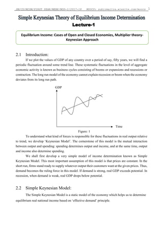
  • 1. SM/CU/MCOM/FIRST YEAR/MEBE/MOD-I/2017-18 MOOCS: subirmaitra.wixsite.com/moocs 1 2.1 Introduction: If we plot the values of GDP of any country over a period of say, fifty years, we will find a periodic fluctuation around some trend line. These systematic fluctuations in the level of aggregate economic activity is known as business cycles consisting of booms or expansions and recessions or contraction. The long run model of the economy cannot explain recession or boom when the economy deviates from its long run path. GDP Time Figure: 1 To understand what kind of forces is responsible for these fluctuations in real output relative to trend, we develop ‘Keynesian Model’. The cornerstone of this model is the mutual interaction between output and spending: spending determines output and income, and at the same time, output and income also determine spending. We shall first develop a very simple model of income determination known as Simple Keynesian Model. This most important assumption of this model is that prices are constant. In the short run, firms stand ready to supply whatever output their customers want at the given prices. Thus, demand becomes the ruling force in this model. If demand is strong, real GDP exceeds potential. In recession, when demand is weak, real GDP drops below potential. 2.2 Simple Keynesian Model: The Simple Keynesian Model is a static model of the economy which helps us to determine equilibrium real national income based on ‘effective demand’ principle. Equilibrium Income: Cases of Open and Closed Economies, Multiplier theory- Keynesian Approach Lecture-1
  • 2. SM/CU/MCOM/FIRST YEAR/MEBE/MOD-I/2017-18 MOOCS: subirmaitra.wixsite.com/moocs 2 2.2.1 Assumptions: (i) One-sector model: The SKM is a one-sector model which includes only the goods market. (ii) Absence of monetary sector: There is no monetary sector in the SKM. (iii) Static model: The SKM is a static model. The model solves for static equilibrium level of real output, which is the value of real output that has no tendency to change once it has been established. (iv) Closed economy with or without Government: The SKM assumes a closed economy (i.e. without foreign trade) with or without Government. (v) Constant prices: In stark contrast to the quantity theory model, the SKM assumes an exogenously fixed price level. (vi) Short-run model: The model is a short-run model and determines the value of real national output for a particular period of time, such as a year. (vii) Fixed stock of capital and labour: The model assumes that both the stock of capital and the labour force, which when fully utilised determine the maximum level of real output the economy can produce, are constant. (viii) Profit maximization: An underlying behavioural assumption of the model is that firms act as profit maximisers. If demand for their output exceeds supply, firms increase production, providing there are spare resources put to work. Conversely if supply exceeds demand, firms reduce output. (ix) Effective demand principle: The SKM is based on Keynesian ‘effective demand principle’. According to this principle, since commodities are necessarily produced for a market, the size of the market must regulate the level of commodity production. Put differently, effective demand refers to that level of the value of aggregate output which, if produced and paid out as income, will be matched by an equivalent amount of expenditure. 2.3 Equilibrium Income (AD—AS Approach): Equilibrium in the SKM requires that the supply of real national output, Y, equals the quantity of national output which people wish to buy, E. The condition for static equilibrium in this model is therefore Y = E ..............(1)
  • 3. SM/CU/MCOM/FIRST YEAR/MEBE/MOD-I/2017-18 MOOCS: subirmaitra.wixsite.com/moocs 3 where E is the ‘desired’ Aggregate Demand or, alternatively, ‘Planned Expenditure’. Alternatively, we can interpret Y as ‘Aggregate Supply’ or ‘Actual Expenditure’ in the economy and rewrite the above condition as Actual Expenditure (Aggregate Supply) = Planned Expenditure (Aggregate Demand) …(2) 2.4 Simple Keynesian Model without Government and Foreign Trade: We now discuss SKM without government and foreign trade. Thus the economy is closed one without any government expenditure (G) as well as taxes (T). 2.4.1 Aggregate Demand (Planned Expenditure) in SKM without Government: Aggregate Demand or planned expenditure in SKM without government is composed of real consumption expenditure C, and real investment expenditure, I. 2.4.2 Consumption Function: Although many factors affect consumption, aggregate disposable income is the most important one. Consumption is assumed to vary directly with income (Y). Specifically, consumption is assumed to increase as income increases, with the increase in consumption being less than the increase in income. In equation form, the consumption function is C = C0 + c Y (C0 >0, 0<c<l) ….......(3) where C and Y represent real consumption and real income, respectively. The equation indicates that consumption is a linear function of disposable income. In the equation, C0 and c are constants, called parameters. Consumption C and income Y are variables. The constant C0 is called autonomous consumption or ‘subsistence consumption’. When Y = 0, C = C0. It is that level of consumption which people must have in order to subsist even if income level falls to zero and it is exogenously given. The parameter c, called the marginal propensity to consume or MPC, is the slope of the consumption function. If ∆Y denotes a change in income and ∆C denotes the change in consumption associated with the change in income, the MPC, equals ∆C / ∆Y. For example, if Y increases by Rs.200 and, as a result, consumption increases by Rs.150, the MPC is 150/200 = 0.75. Thus consumption increases as Y increases, but by a smaller amount. This implies that, the MPC, must be between 0 and 1, an assumption which is in accord with the empirical evidence. We can graphically represent (Fig:2) the consumption function. We know that ' C0 ' is the intercept parameter and 'c' is the slope parameter. Once the intercept and slope are specified, a straight line is completely determined. For example, if C0 =100 and c = 0.75, the function will start at C0 = 100 and have a slope c = 0.75. If there is a change in C0, the consumption function will shift so that
  • 4. SM/CU/MCOM/FIRST YEAR/MEBE/MOD-I/2017-18 MOOCS: subirmaitra.wixsite.com/moocs 4 the new function is parallel to the old. If there is a change in c, the function will rotate about the intercept, C0 and will be either steeper or flatter. C0 Figure: 2 2.4.3 Investment Function: Like consumption, investment depends on many factors, including interest rates. In the SKM, however, investment is assumed to be an autonomous or exogenous variable -- a variable whose value is determined outside the model. Thus, investment is a constant, I0 (I0 >0). Since investment is assumed to be constant at the Ī level, the investment function is I = I0 (I0 >0) ………(4) where I represents real investment and Ī represents a given, positive level of investment. Suppose I0 equals Rs. 50. With investment on the vertical axis and income on the horizontal, the investment function is plotted as the horizontal line in Figure: 3,indicating that investment does not vary with the level of income. C = C0 + c.Y Income (Y) Consumption (C) Investment (I) I = I0 Income (Y) Figure: 3
  • 5. SM/CU/MCOM/FIRST YEAR/MEBE/MOD-I/2017-18 MOOCS: subirmaitra.wixsite.com/moocs 5 2.5 Equilibrium Income in Simple Keynesian Model without Government: The economy in the SKM is said to be in equilibrium when Actual Expenditure (Aggregate Supply) = Planned Expenditure (Aggregate Demand) i.e. Y = C + I ….(5)  Y = C0 + c Y + I0  Y = C0+ c.Y + I0  Y = C0 + c.Y + I0 …..(6) By rearranging we get: YE = [{C0 + I0} / (1 – c)] ….(7) where YE is the equilibrium level of income in the SKM without government -- that level of income which makes actual expenditure (AD) in the economy same as planned expenditure (AS). 2.6 Graphical Illustration: The aggregate supply-aggregate demand approach is developed graphically in Figure: . Aggregate supply, the output of goods and services, is depicted by the 45° line. With the same scales on both axes, output on the vertical axis equals output or income on the horizontal axis for all points on the 45° line. The 45° line is not a 'true' aggregate supply curve. For example, it indicates that any amount, from 0 to infinity, may be produced. This is not possible; production is limited by the nation's resources and its technology. Nevertheless, in the development of the model, it is helpful to think of the 45° line as an aggregate supply curve. YE Figure: 4 Aggregate demand represents society's demand for goods and services. With no foreign trade sector, it consists of the demand for consumer goods and services, the demand for investment goods and government purchases. Consequently, AD = C + c.Y + I Aggregate Supply (Y) Aggregate Demand (AD)
  • 6. SM/CU/MCOM/FIRST YEAR/MEBE/MOD-I/2017-18 MOOCS: subirmaitra.wixsite.com/moocs 6 AD = C + I = (C0 + c.Y + I0 ) Graphically, the aggregate demand line is the positively sloped line AD whose intercept is equal to (C0 + I0 ) and slope is equal to 0 < c < 1. With the 45° line representing ‘aggregate supply’ or ‘actual expenditure’ and the AD line representing ‘aggregate demand’ or ‘planned expenditure’, the equilibrium level of income is YE. Income level YE is the equilibrium level since it is the only level for which aggregate supply equals aggregate demand. At income levels greater than YE, aggregate supply (represented by the 45° line) is greater than aggregate demand (represented by the AD line), and income has a tendency to fall. At income levels less than YE, aggregate supply is less than aggregate demand, and income has a tendency to rise. When AS > AD, Y tends to fall because of the unplanned inventory accumulation by the firms (Iu = ∆inv. > 0), as producers are unable to sell their products. When AD > AS, Y tends to increase because of the unplanned depletion in inventories by the firms (Iu = ∆inv. < 0) to meet increased demand. When AD = AS, Y is at its equilibrium level. Since income tends to fall when AS > AD and to rise when AD > AS, income eventually gravitates to its equilibrium level => stable equilibrium. 2.7 Economic Explanation: If the nation's income (output) equals the equilibrium income (output), firms will be able to sell their entire output. Consequently, no incentive exists for them to alter their production and income remains at the equilibrium level. If the nation's output exceeds the equilibrium output, firms are unable to sell their entire output and experience a buildup in their inventories. An incentive exists, therefore, for them to reduce production. As a result, output falls until it equals the demand for goods and services. Similarly, if the nation's output is less than the demand for goods and services, firms sell more than they are producing and experience a depletion of their inventories. An incentive exists, therefore, for them to increase production. As a result, output rises until it equals the demand for goods and services. 2.8 Equilibrium Income in Simple Keynesian Model with Government: We now discuss SKM with government but without foreign trade. Thus the economy is closed one but government plays an active role in the economy. Thus, government spends (G) as well as taxes (T).
  • 7. SM/CU/MCOM/FIRST YEAR/MEBE/MOD-I/2017-18 MOOCS: subirmaitra.wixsite.com/moocs 7 2.8.1 Aggregate Demand (Planned Expenditure) in SKM with Government: Aggregate Demand or planned expenditure in SKM with government is composed of real consumption expenditure C, and real investment expenditure, I and real government purchases, G. Consumption and investment functions have been discussed above. But the presence of government makes certain changes in the C function. 2.8.2 The Consumption Function in SKM with government: In the presence of a government, imposing taxes on income, consumption is assumed to vary directly with disposable income (YD). Specifically, consumption is assumed to increase as disposable income increases, with the increase in consumption being less than the increase in disposable income. In equation form, the consumption function is C = C0 + c YD (C0 >0, 0<c<l) ….....(8) where C and YD represent real consumption and real disposable income, respectively. The equation indicates that consumption is a linear function of disposable income. In the equation, C0 and c are constants, called parameters. Consumption, C, and income, Y, are variables. Disposable income (YD) is equal to income plus transfers (TR) less taxes(T): YD ≡ Y + TR – T …….(9) The constant C0 is called autonomous consumption or ‘subsistence consumption’. When YD = 0, C = C0. It is that level of consumption which people must have in order to subsist even if income level falls to zero and it is exogenously given. The parameter c, called the marginal propensity to consume or MPC, is the slope of the consumption function. We can graphically represent the consumption function same as in Figure:2. 2.8.3 Government purchases: Like investment, real government purchases are also exogenously given. Government expenditure includes such items as national defense expenditures, salaries of government employees etc. G is a policy variable, whose value is determined by the Government. In a democratic country like ours, G is decided after prolonged discussion in the Parliament. Hence we can write: G = G0 ……..(10) 2.8.4 Taxes and Transfers: Transfers (or transfer payments) are those payments that are made to people without their providing a current service in exchange. Typical transfer payments are social security benefits and unemployment benefits. In the SKM, transfers are assumed to be exogenously given i.e. TR = TR0 ……(11) Taxes are compulsory payments to be made by the citizens of a country. Taxes may or may not depend on the income. For example,
  • 8. SM/CU/MCOM/FIRST YEAR/MEBE/MOD-I/2017-18 MOOCS: subirmaitra.wixsite.com/moocs 8 (i) If the taxes are lump-sum, T = 𝑇̅ (𝑇̅ >0) ……(12) (ii) If taxes are function of income: T = T(Y), 0< TY <1 ……(13) (iii) If taxes are proportional to income: T = t. Y, 0 < t < 1 …..(14) (iv) If taxes are partly lump-sum and partly proportional: T = 𝑇̅ + t.Y (𝑇̅> 0; 0 < t < 1) .…(15) Note that ∂T/ ∂Y = TY represents the change in T due to one unit change in Y which is the tax rate. Under proportional income tax, ∂T/ ∂Y = t where ‘t’ is the fixed tax rate such that 0 < t < 1. Obviously, T and t are decided by the Government and is therefore exogenously given. 2.8.5 Equilibrium Income in Simple Keynesian Model with Government: The economy in the SKM is said to be in equilibrium when Actual Expenditure (Aggregate Supply) = Planned Expenditure (Aggregate Demand) i.e. Y = C + I + G ….(16)  Y = C0 + c YD + I0 + G0  Y = C0 + c.( Y + TR0 –T0) + I0 + G0  Y = C0 + c.(Y + TR0 – t .Y) + I0 + G0 (assuming proportional taxes) …..(17) By rearranging we get:  YE = [ 1 / {1 – c(1-- t)}]{ C0 + c.TR0+ I0 + G0} ….(18) where YE is the equilibrium level of income-- that level of income which makes actual expenditure(AD) in the economy same as planned expenditure(AS). Alternatively, the AD equation can also be written as:  AD = { C0 + c.TR0 + I0 + G0} + c.(Y – t .Y) = 𝐴̅ + c (1 – t) Y …..(19) where 𝐴̅ = { C0 + c.TR0 + Ī + G0} is the autonomous part of AD. The equilibrium condition: Y = 𝐴̅ + c (1 – t) Y => YE = [ 1 / {1 – c(1-- t)}]. 𝐴̅ ……(20) If the nation's income (output) equals the equilibrium income (output), firms will be able to sell their entire output. Consequently, no incentive exists for them to alter their production and income remains at the equilibrium level. If the nation's output exceeds the equilibrium output, firms are unable to sell their entire output and experience a buildup in their inventories. An incentive exists, therefore, for them to reduce
  • 9. SM/CU/MCOM/FIRST YEAR/MEBE/MOD-I/2017-18 MOOCS: subirmaitra.wixsite.com/moocs 9 production. As a result, output falls until it equals the demand for goods and services. Similarly, if the nation's output is less than the demand for goods and services, firms sell more than they are producing and experience a depletion of their inventories. An incentive exists, therefore, for them to increase production. As a result, output rises until it equals the demand for goods and services. 2.8.6 Graphical Illustration: The determination of equilibrium income in SKM with government is shown graphically in Figure: . Aggregate supply, the output of goods and services, is depicted by the 45° line. With the same scales on both axes, output on the vertical axis equals output or income on the horizontal axis for all points on the 45° line. The 45° line is not a 'true' aggregate supply curve. For example, it indicates that any amount, from 0 to infinity, may be produced. This is not possible; production is limited by the nation's resources and its technology. Nevertheless, in the development of the model, it is helpful to think of the 45° line as an aggregate supply curve. Aggregate demand represents society's demand for goods and services. With no foreign trade sector, it consists of the demand for consumer goods and services, the demand for investment goods and government purchases. Consequently, AD = C + I + G  = {C0 + c.TR0 + I0 + G0} + c.(Y – t .Y) = 𝐴̅ + c (1 – t) Y Graphically, the aggregate demand line is the positively sloped line AD whose intercept is equal to A and slope is equal to 0 < c (1 – t) < 1. YE Fig: 5 With the 45° line representing ‘aggregate supply’ or ‘actual expenditure’ and the AD line representing ‘aggregate demand’ or ‘planned expenditure’, the equilibrium level of income is YE. AD = 𝑨̅ + c (1 – t) Y Aggregate Supply (Y) Aggregate Demand (AD)
  • 10. SM/CU/MCOM/FIRST YEAR/MEBE/MOD-I/2017-18 MOOCS: subirmaitra.wixsite.com/moocs 10 Income level YE is the equilibrium level since it is the only level for which aggregate supply equals aggregate demand. At income levels greater than YE, aggregate supply (represented by the 45° line) is greater than aggregate demand (represented by the AD line), and income has a tendency to fall. At income levels less than YE, aggregate supply is less than aggregate demand, and income has a tendency to rise. When AS > AD, Y tends to fall because of the unplanned inventory accumulation by the firms ( Iu = ∆inv. > 0), as producers are unable to sell their products. When AD > AS, Y tends to increase because of the unplanned depletion in inventories by the firms ( Iu = ∆inv. < 0) to meet increased demand. When AD = AS, Y is at its equilibrium level. Since income tends to fall when AS > AD and to rise when AD > AS, income eventually gravitates to its equilibrium level => stable equilibrium. 2.9 Is equilibrium income = full employment income? In the SKM with or without government, the equilibrium level of income may or may not represent a full-employment level. That is, full-employment may or may not exist at the equilibrium level of income. Unemployment may exist at the equilibrium level of income because, for the model in question, the equilibrium level of income is merely the level where intended investment equals saving or, alternatively, aggregate supply equals aggregate demand. Here, we assume that unemployment exists so that increases in aggregate demand result in increases in production. 2.10 Existence of Equilibrium: Once the equilibrium in the SKM is established one may question whether is exists or not. The equilibrium exists if AD and AS curves intersect each other in positive quadrant so that YE > 0. For this sufficient condition (with 𝐴̅ >0) is that AD must be flatter than AS. Since slope of AD is c (1 – t) and that of AS is 1, the sufficient condition for the existence of equilibrium is c (1 – t) < 1 which always holds as 0 < c (1 – t) < 1 (Fig: 5). That equilibrium would not exist if c (1 – t) > 1 may be seen from the Fig: where AD is steeper than AS so that no intersection is possible in the positive quadrant. 2.11 Stability of Equilibrium: That equilibrium in the SKM is stable can be realized from the fact that a disturbance in the equilibrium causing the income Y to be different from YE, generates such forces which brings back the economy back to equilibrium once again. With 𝐴̅ > 0, the sufficient condition for this stability is that AD is flatter than AS i.e. c (1 – t) < 1. Since 0 < c (1 – t) < 1 always, the SKM gives a stable equilibrium. The economic interpretation of this stability is: When AD < AS
  • 11. SM/CU/MCOM/FIRST YEAR/MEBE/MOD-I/2017-18 MOOCS: subirmaitra.wixsite.com/moocs 11  Unplanned accumulation of inventories by the firms (Δinv >0)  Unplanned or unintended investment ( Iu) > 0  Reduction in production by the firms,  Y falls till Y = YE Again when AD > AS  Unplanned decumulation of inventories by the firms (Δinv < 0)  Unplanned or unintended investment ( Iu) < 0  Increase in production by the firms,  Y increases till Y = YE  Stable Equilibrium.