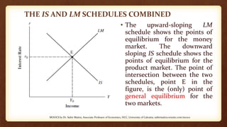
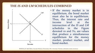
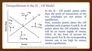
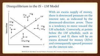
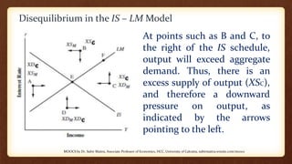
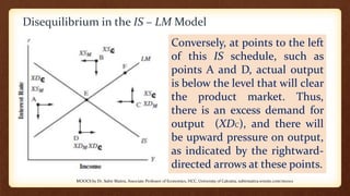
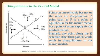
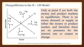
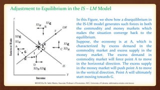
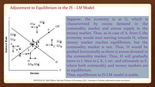
MOOCS by Dr. Subir Maitra
Course Name: M.Com Year: First
Session: 2017-18
Paper- 1.3
Macroeconomics and Business Environment
Module: One
Lecture-11
Department of Commerce
University of Calcutta
MOOCS by Dr. Subir Maitra, Associate Professor of Economics, HCC, subirmaitra.wixsite.com/moocs
General Equilibrium: Aspects of Closed Economy--
Commodity Market and Money Market Equilibrium--
IS-LM Approach.
IS-LM MODEL: GENERAL EQUILIBRIUM,
ADJUSTMENT TO EQUILIBRIUM
MOOCS by Dr. Subir Maitra, Associate Professor of Economics, HCC, subirmaitra.wixsite.com/moocs
THE IS AND LM SCHEDULES COMBINED
‱ The upward-sloping LM
schedule shows the points of
equilibrium for the money
market. The downward
sloping IS schedule shows the
points of equilibrium for the
product market. The point of
intersection between the two
schedules, point E in the
figure, is the (only) point of
general equilibrium for the
two markets.
MOOCS by Dr. Subir Maitra, Associate Professor of Economics, HCC, University of Calcutta, subirmaitra.wixsite.com/moocs
THE IS AND LM SCHEDULES COMBINED
‱ If the money market is in
equilibrium, the bond market
must also be in equilibrium.
Thus, the interest rate and
income level at the
intersection of the IS and LM
schedules in the Figure
denoted r0 and Y0, are values
that produce a simultaneous
equilibrium for the money
market, product market, and
bond market.
MOOCS by Dr. Subir Maitra, Associate Professor of Economics, HCC, University of Calcutta, subirmaitra.wixsite.com/moocs
Disequilibrium in the IS – LM Model
In the IS – LM model, points other
than the point of intersection of the
two schedules are not points of
equilibrium.
First, consider points above the LM
schedule such as points A and B. At all
points above the LM schedule, there
will be an excess supply of money
(XSM). At the level of income for
either point A or B, the corresponding
interest rate is too high for money
market equilibrium.
MOOCS by Dr. Subir Maitra, Associate Professor of Economics, HCC, University of Calcutta, subirmaitra.wixsite.com/moocs
Disequilibrium in the IS – LM Model
With an excess supply of money,
there is downward pressure on the
interest rate, as indicated by the
downward-direction arrow. There
is a tendency to move toward the
LM schedule. Conversely, at points
below the LM schedule, such as
points C and D, there will be an
excess demand for money (XDM)
and consequently upward pressure
on the interest rate.
MOOCS by Dr. Subir Maitra, Associate Professor of Economics, HCC, University of Calcutta, subirmaitra.wixsite.com/moocs
Disequilibrium in the IS – LM Model
At points such as B and C, to
the right of the IS schedule,
output will exceed aggregate
demand. Thus, there is an
excess supply of output (XSC),
and therefore a downward
pressure on output, as
indicated by the arrows
pointing to the left.
MOOCS by Dr. Subir Maitra, Associate Professor of Economics, HCC, University of Calcutta, subirmaitra.wixsite.com/moocs
Disequilibrium in the IS – LM Model
Conversely, at points to the left
of this IS schedule, such as
points A and D, actual output
is below the level that will clear
the product market. Thus,
there is an excess demand for
output (XDC), and there will
be upward pressure on output,
as indicated by the rightward-
directed arrows at these points.
MOOCS by Dr. Subir Maitra, Associate Professor of Economics, HCC, University of Calcutta, subirmaitra.wixsite.com/moocs
Disequilibrium in the IS – LM Model
Points on one schedule but not on
the other are disequilibrium. A
point such as F is a point of
equilibrium for the money market
but a point of excess supply for the
product market.
Similarly, any point along the IS
schedule other than point E would
result in disequilibrium in the
money market.
MOOCS by Dr. Subir Maitra, Associate Professor of Economics, HCC, University of Calcutta, subirmaitra.wixsite.com/moocs
Disequilibrium in the IS – LM Model
Only at point E are both the
money and product markets
in equilibrium. There is no
excess demand or supply in
either the money or product
market, and therefore there
are no pressures for the
interest rate or output to
change.
MOOCS by Dr. Subir Maitra, Associate Professor of Economics, HCC, University of Calcutta, subirmaitra.wixsite.com/moocs
Adjustment to Equilibrium in the IS – LM Model
In this Figure, we show how a disequilibrium in
the IS-LM model generates such forces in both
the commodity and money markets which
makes the situation converge back to the
equilibrium.
Suppose, the economy is at A, which is
characterized by excess demand in the
commodity market and excess supply in the
money market. The excess demand in
commodity market will force point A to move
in the horizontal direction. The excess supply
in the money market will push point A to move
in the vertical direction. Point A will ultimately
start moving towards G.
MOOCS by Dr. Subir Maitra, Associate Professor of Economics, HCC, University of Calcutta, subirmaitra.wixsite.com/moocs
Adjustment to Equilibrium in the IS – LM Model
Suppose, the economy is at G, which is
characterized by excess demand in the
commodity market and excess supply in the
money market. Thus, as in case of A, from G the
economy would start moving towards H, where
money market reaches equilibrium, but the
commodity market is not. Thus, H would be
pushed horizontally as there is excess demand in
the commodity market. Thus, H will gradually
move to I, then to J, K, L etc. and ultimately to E,
where both commodity and money markets are
in equilibrium.
Thus, equilibrium in IS-LM model is stable.
MOOCS by Dr. Subir Maitra, Associate Professor of Economics, HCC, University of Calcutta, subirmaitra.wixsite.com/moocs
End of Lecture 11
MOOCS by Dr. Subir Maitra, Associate Professor of Economics, HCC, subirmaitra.wixsite.com/moocs

IS-LM Model 3

  • 1.
    MOOCS by Dr.Subir Maitra Course Name: M.Com Year: First Session: 2017-18 Paper- 1.3 Macroeconomics and Business Environment Module: One Lecture-11 Department of Commerce University of Calcutta MOOCS by Dr. Subir Maitra, Associate Professor of Economics, HCC, subirmaitra.wixsite.com/moocs
  • 2.
    General Equilibrium: Aspectsof Closed Economy-- Commodity Market and Money Market Equilibrium-- IS-LM Approach. IS-LM MODEL: GENERAL EQUILIBRIUM, ADJUSTMENT TO EQUILIBRIUM MOOCS by Dr. Subir Maitra, Associate Professor of Economics, HCC, subirmaitra.wixsite.com/moocs
  • 3.
    THE IS ANDLM SCHEDULES COMBINED ‱ The upward-sloping LM schedule shows the points of equilibrium for the money market. The downward sloping IS schedule shows the points of equilibrium for the product market. The point of intersection between the two schedules, point E in the figure, is the (only) point of general equilibrium for the two markets. MOOCS by Dr. Subir Maitra, Associate Professor of Economics, HCC, University of Calcutta, subirmaitra.wixsite.com/moocs
  • 4.
    THE IS ANDLM SCHEDULES COMBINED ‱ If the money market is in equilibrium, the bond market must also be in equilibrium. Thus, the interest rate and income level at the intersection of the IS and LM schedules in the Figure denoted r0 and Y0, are values that produce a simultaneous equilibrium for the money market, product market, and bond market. MOOCS by Dr. Subir Maitra, Associate Professor of Economics, HCC, University of Calcutta, subirmaitra.wixsite.com/moocs
  • 5.
    Disequilibrium in theIS – LM Model In the IS – LM model, points other than the point of intersection of the two schedules are not points of equilibrium. First, consider points above the LM schedule such as points A and B. At all points above the LM schedule, there will be an excess supply of money (XSM). At the level of income for either point A or B, the corresponding interest rate is too high for money market equilibrium. MOOCS by Dr. Subir Maitra, Associate Professor of Economics, HCC, University of Calcutta, subirmaitra.wixsite.com/moocs
  • 6.
    Disequilibrium in theIS – LM Model With an excess supply of money, there is downward pressure on the interest rate, as indicated by the downward-direction arrow. There is a tendency to move toward the LM schedule. Conversely, at points below the LM schedule, such as points C and D, there will be an excess demand for money (XDM) and consequently upward pressure on the interest rate. MOOCS by Dr. Subir Maitra, Associate Professor of Economics, HCC, University of Calcutta, subirmaitra.wixsite.com/moocs
  • 7.
    Disequilibrium in theIS – LM Model At points such as B and C, to the right of the IS schedule, output will exceed aggregate demand. Thus, there is an excess supply of output (XSC), and therefore a downward pressure on output, as indicated by the arrows pointing to the left. MOOCS by Dr. Subir Maitra, Associate Professor of Economics, HCC, University of Calcutta, subirmaitra.wixsite.com/moocs
  • 8.
    Disequilibrium in theIS – LM Model Conversely, at points to the left of this IS schedule, such as points A and D, actual output is below the level that will clear the product market. Thus, there is an excess demand for output (XDC), and there will be upward pressure on output, as indicated by the rightward- directed arrows at these points. MOOCS by Dr. Subir Maitra, Associate Professor of Economics, HCC, University of Calcutta, subirmaitra.wixsite.com/moocs
  • 9.
    Disequilibrium in theIS – LM Model Points on one schedule but not on the other are disequilibrium. A point such as F is a point of equilibrium for the money market but a point of excess supply for the product market. Similarly, any point along the IS schedule other than point E would result in disequilibrium in the money market. MOOCS by Dr. Subir Maitra, Associate Professor of Economics, HCC, University of Calcutta, subirmaitra.wixsite.com/moocs
  • 10.
    Disequilibrium in theIS – LM Model Only at point E are both the money and product markets in equilibrium. There is no excess demand or supply in either the money or product market, and therefore there are no pressures for the interest rate or output to change. MOOCS by Dr. Subir Maitra, Associate Professor of Economics, HCC, University of Calcutta, subirmaitra.wixsite.com/moocs
  • 11.
    Adjustment to Equilibriumin the IS – LM Model In this Figure, we show how a disequilibrium in the IS-LM model generates such forces in both the commodity and money markets which makes the situation converge back to the equilibrium. Suppose, the economy is at A, which is characterized by excess demand in the commodity market and excess supply in the money market. The excess demand in commodity market will force point A to move in the horizontal direction. The excess supply in the money market will push point A to move in the vertical direction. Point A will ultimately start moving towards G. MOOCS by Dr. Subir Maitra, Associate Professor of Economics, HCC, University of Calcutta, subirmaitra.wixsite.com/moocs
  • 12.
    Adjustment to Equilibriumin the IS – LM Model Suppose, the economy is at G, which is characterized by excess demand in the commodity market and excess supply in the money market. Thus, as in case of A, from G the economy would start moving towards H, where money market reaches equilibrium, but the commodity market is not. Thus, H would be pushed horizontally as there is excess demand in the commodity market. Thus, H will gradually move to I, then to J, K, L etc. and ultimately to E, where both commodity and money markets are in equilibrium. Thus, equilibrium in IS-LM model is stable. MOOCS by Dr. Subir Maitra, Associate Professor of Economics, HCC, University of Calcutta, subirmaitra.wixsite.com/moocs
  • 13.
    End of Lecture11 MOOCS by Dr. Subir Maitra, Associate Professor of Economics, HCC, subirmaitra.wixsite.com/moocs