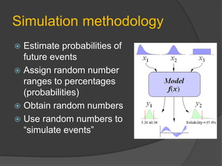
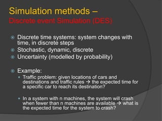
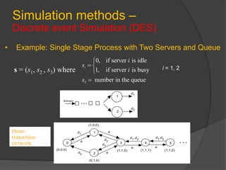
This document discusses static and dynamic models, deterministic and stochastic models, and various methods for studying systems with uncertainty. Deterministic models use differential equations to exactly predict outcomes, while stochastic models use random variables and can only compute probabilities. Numerical methods and simulation are introduced as ways to study more complex systems. Simulation models represent real systems and allow experiments to be performed faster and safer. Monte Carlo methods and discrete event simulation are discussed as techniques for simulation.

1. Static - Dynamic
Anna Maria Sri Asih
Department of Mechanical & Industrial Engineering
Gadjah Mada University

2. Introduction
 Deterministic models:
 expressed in terms of differential equations
 can exactly predict the development of a system based
on initial and boundary conditions
 Stochastic models
 use random variables
 outcomes are uncertain
 can only compute the probabilities of possible outcomes
Example:
throwing dice ( random experiment)
 outcome of a toss: initial conditions & external forces
 uncertain ?

3. How to study system?

4. How to study system?
 Analytic solution
 know how the model will behave iner any circumstances.
 closed form solution
 simple models
 Numerical methods
 More complex system
 example: Runge-Kutta method
Starts with the initial values of the variables, then use the
equations to figure out the changes In these variables over a very brief
time period
 repetition / iteration
 result: long list numbers, NOT equation
 Simulation
 even more complex system
 deals with uncertainty
 ”Calculate when you can, simulate when you can’t!”

5. Simulation models
 Model of the real system
 Faster, cheaper, or safer to perform
experiments on the model
 Computer simulation may use formulas,,
programming statements, or other means
to express math relationships between
inputs and outputs.
 Dealing with uncertainty  include
uncertain variables  random values from
a distribution.
 Simulation run includes many trials

6. Advantages of simulation
 Allows the study of complex, real-world systems (which
otherwise cannot be studied)
 Estimates performance of existing system under ‘projected’ /
different operating conditions
 Compares alternative proposed system designs
 Better control over experimental conditions
 Compress time, expand time
 Overall, if done correctly, simulation gives planners unlimited
freedom to try out different ideas for design and improvement
Disadvantages and pitfalls of
simulation
 Failure to produce exact results (only estimates)
 Costs of developing simulation models can be
expensive and time consuming

7. Simulation methodology
 Estimate probabilities of
future events
 Assign random number
ranges to percentages
(probabilities)
 Obtain random numbers
 Use random numbers to
“simulate events”

8. Simulation life cycle
Ayani, R., 2003

9. Building a valid and credible
simulation model
 Picture
verification asks “ Was the model made right? ”
validation asks “ Was the right model made? ”
accreditation asks “ Is the model the right one for the job? ”

10. Simulation methods – Monte Carlo
It is a method that
methods for solving
various kinds of
computational problems
by using random numbers

11. Simulation methods – Monte Carlo
“Find the value of ”
 Use “hit and miss” method
 The area of square = (2r)2
 The area of circle = r2

𝑎𝑟𝑒𝑎 𝑜𝑓 𝑠𝑞𝑢𝑎𝑟𝑒
𝑎𝑟𝑒𝑎 𝑜𝑓 𝑐𝑖𝑟𝑐𝑙𝑒
=
4𝑟2
𝑟2 =
4

  = 4 ∗
𝑎𝑟𝑒𝑎 𝑜𝑓 𝑐𝑖𝑟𝑐𝑙𝑒
𝑎𝑟𝑒𝑎 𝑜𝑓 𝑠𝑞𝑢𝑎𝑟𝑒
=
𝑛𝑢𝑚𝑏𝑒𝑟 𝑜𝑓 𝑑𝑜𝑡𝑠 𝑖𝑛𝑠𝑖𝑑𝑒 𝑐𝑖𝑟𝑐𝑙𝑒
𝑡𝑜𝑡𝑎𝑙 𝑛𝑢𝑚𝑏𝑒𝑟 𝑜𝑓 𝑑𝑜𝑡𝑠
r

12. Simulation methods – Monte Carlo
“Find the value of ”
 Use “hit and miss” method
 The area of square = (2r)2
 The area of circle = r2

𝑎𝑟𝑒𝑎 𝑜𝑓 𝑠𝑞𝑢𝑎𝑟𝑒
𝑎𝑟𝑒𝑎 𝑜𝑓 𝑐𝑖𝑟𝑐𝑙𝑒
=
4𝑟2
𝑟2 =
4

  = 4 ∗
𝑎𝑟𝑒𝑎 𝑜𝑓 𝑐𝑖𝑟𝑐𝑙𝑒
𝑎𝑟𝑒𝑎 𝑜𝑓 𝑠𝑞𝑢𝑎𝑟𝑒
=
𝑛𝑢𝑚𝑏𝑒𝑟 𝑜𝑓 𝑑𝑜𝑡𝑠 𝑖𝑛𝑠𝑖𝑑𝑒 𝑐𝑖𝑟𝑐𝑙𝑒
𝑡𝑜𝑡𝑎𝑙 𝑛𝑢𝑚𝑏𝑒𝑟 𝑜𝑓 𝑑𝑜𝑡𝑠
r

13. Simulation methods – Monte Carlo
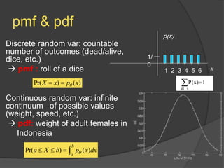
“Birthday problem”
 Out of a group of 100 people, 2 people share a brithday
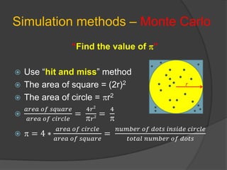
 Use “hit and miss” method
1. Pick 30 random numbers in the rang [1,365], each number
represent a day in a year
2. Check to see if any of the 30 random numbers are equal
3. Go back to step [1] and repeat 10,000 times
4. Report the fraction of trials that have matching birthdays

14. Simulation methods – Monte Carlo
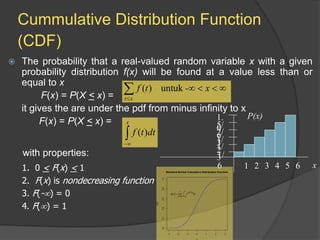
“Birthday problem”
 Out of a group of 100 people, 2 people share a brithday
 Use “sampling from distribution” method
1. Suppose we have the cdf of people’s birthday, F(x)
2. People’s birthday is represented as x = [1, 365]
3. Generate a random values, z, from U [0,1]
4. Compute x = F-1(z)
5. Check to see if any of the 30 random numbers are equal
6. Go back to step [3,4] and repeat 10,000 times
7. Report the fraction of trials that have matching birthdays
Many kinds of sampling, e.g.:
• Simple sampling
• Importance sampling
• Stratified sampling
• Non-stratified sampling
• Cluster sampling
• Latin hypercube
Output from Monte Carlo
can form a distribution too !

15. Simulation methods –
Discrete event Simulation (DES)
 Discrete time systems: system changes with
time, in discrete steps
 Stochastic, dynamic, discrete
 Uncertainty (modelled by probability)
 Example:
 Traffic problem: given locations of cars and
destinations and traffic rules  the expected time for
a specific car to reach its destination?
 In a system with n machines, the system will crash
when fewer than n machines are available  what is
the expected time for the system to crash?

16. Simulation methods –
Discrete event Simulation (DES)
 Example: Single-server queue
 Estimate expected average delay in queue (line, not service)
 State variables
○ Status of server (idle, busy) – needed to decide what to do with an
arrival
○ Current length of the queue – to know where to store an arrival that
must wait in line
○ Time of arrival of each customer now in queue – needed to compute
time in queue when service starts
 Events
○ Arrival of a new customer
○ Service completion (and departure) of a customer
○ Maybe – end-simulation event (a “fake” event) – whether this is an
event depends on how simulation terminates (a modeling decision)

17. Status
shown is
after all
changes
have
been
made in
each
case …
Interarrival times: 0.4, 1.2, 0.5, 1.7, 0.2, 1.6, 0.2, 1.4, 1.9, …
Service times: 2.0, 0.7, 0.2, 1.1, 3.7, 0.6, …
Interarrival times: 0.4, 1.2, 0.5, 1.7, 0.2, 1.6, 0.2, 1.4, 1.9, …
Service times: 2.0, 0.7, 0.2, 1.1, 3.7, 0.6, …

18. Interarrival times: 0.4, 1.2, 0.5, 1.7, 0.2, 1.6, 0.2, 1.4, 1.9, …
Service times: 2.0, 0.7, 0.2, 1.1, 3.7, 0.6, …
Final output performance measures:
Average delay in queue = 5.7/6 = 0.95 min./cust.
Time-average number in queue = 9.9/8.6 = 1.15 custs.
Server utilization = 7.7/8.6 = 0.90 (dimensionless)

19. • Example: Single Stage Process with Two Servers and Queue
1
2
Arrivals
…
d1
d2
s = (s1, s2 , s3) where
0
1
2
3 4 5
(0,0,0)
(0,1,0)
(1,1,0) (1,1,1) (1,1,2)
(1,0,0)
• • •
a
a
a
a a
d1
d2
d2
d2
d2
d1
d1
d1
, ,
State-
transition
network
3
0, if server is idle
1, if server is busy
number in the queue
i
i
s
i
s

 


i = 1, 2
Simulation methods –
Discrete event Simulation (DES)

20. Simulation methods –
Discrete event Simulation (DES)
 Example: repair problem
n machines are needed to keep an operation.
There are s spare machines.
The machines in operation fail according to some unknown distribution
(e.g. exponential, Poisson, uniform, etc., with a known mean).
When a machine fails it is sent to repair shop and the time to fix is a
random variable that follows a known distribution.
System crashes when fewer than n machines are available
What is the expected time for the system to crash?

21. Simulation methods –
Discrete event Simulation (DES)
n = number of working machines needed
S = number of spares available

22. Simulation methods – Continuous
 Continuous time model:
 state variables may change
continuously, e.g. temperature in a class
room, the level of water in a tank
 used extensively in mechanical, chemical,
and electrical engineering
 Example:
 the level of temperature of a liquid
 the level of temperature in a classroom
 the level of water in a tank
 the level of drug concentration in body

23. Simulation methods – Hybrid
 Hybrid : combined discrete / continuous
model
 Some variables in the system model are
discrete and some continuous
 Example: unloading dock where tankers
queue up to unload their oil through a
pipeline:
 discrete : tanker arrivals
 continuous : flow of oil

24. Random variables
& Stochastic Process
 Random variables:
 variable whose possible values are numerical
outcomes of a random phenomenon
 Types:
Discrete random var: countable number of outcomes
(dead/alive, dice, etc.)
Continuous random var: infinite continuum of
possible values ( weight, speed, etc.)
 Stochastic process:
 a family of random variables

25. Probability functions
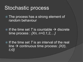
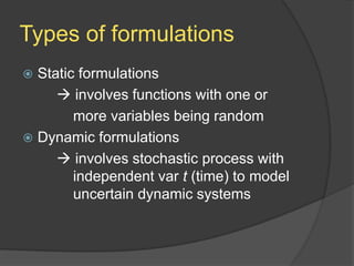
 A probability function maps the possible
values x against their respective
probabilities of occurrence, p(x)
 p(x)  [0,1]
 The area under a probability function is
always 1

26. pmf & pdf
Discrete random var: countable
number of outcomes (dead/alive,
dice, etc.)
 pmf : roll of a dice
Continuous random var: infinite
continuum of possible values
(weight, speed, etc.)
 pdf: weight of adult females in
Indonesia
x
p(x)
1/
6
1 4 5 6
2 3
 
x
all
1
P(x)
Pr( ) ( )
X x p x

 
Pr( ) ( )
b
a
a X b p x dx

   

27.  The probability that a real-valued random variable x with a given
probability distribution f(x) will be found at a value less than or
equal to x
F(x) = P(X < x) =
it gives the are under the pdf from minus infinity to x
F(x) = P(X < x) =
with properties:






x
t
x
-
t
f untuk
)
(
1. 0 < F(x) < 1
2. F(x) is nondecreasing function
3. F(-) = 0
4. F() = 1
Cummulative Distribution Function
(CDF)


x
dt
t
f )
(
x
P(x)
1/
6 1 4 5 6
2 3
1/
3
1/
2
2/
3
5/
6
1.
0

28. Stochastic process
 The process has a strong element of
random behaviour
 If the time set T is countable  discrete
time process : {Xn, n=0,1,2,…}
 If the time set T is an interval of the real
line  continuous time process: {X(t),
t0}

29. Types of formulations
 Static formulations
 involves functions with one or
more variables being random
 Dynamic formulations
 involves stochastic process with
independent var t (time) to model
uncertain dynamic systems