SlideShare a Scribd company logo
Mark P. Wason Detail CFD Analysis of NACA 0015 Airfoil AERO406
1
DETAILED CFD ANALYSIS OF NACA 0015 AIRFOIL
(Mid-Project Report – setup and mesh)
MARK P. WASON, Cal Poly ID 007868194
Department of Aerospace Engineering,
California Polytechnic State University
San Luis Obispo, CA 93407
Nomenclature
𝑐 Chord length
𝐢𝑙 Lift coefficient, 2 dimensional
𝐢 𝑑 Drag coefficient, 2 dimensional
𝑙 Lift, 2 dimensional
𝑑 Drag, 2 dimensional
π‘’βˆ— Friction velocity
π‘ˆβˆž Freestream velocity
y Wall spacing
𝑦+
Y-plus value
𝜈 Kinematic viscosity
1 Introduction
This computational fluid dynamics (CFD)
analysis investigates the behaviour of a symmetric
airfoil in climb conditions, directly pertinent to the
undergraduate design competition request for proposal
for the preliminary design of an aerobatic light sport
aircraft (LSA). A NACA 0015 airfoil was selected for
this study for the wealth of data from both CFD and
experimentation available and its possible use directly
or indirectly in the design project.
NACA airfoils have been repeatedly used in CFD
as a baseline for evaluation of turbulence models and
solver performance, as in Sahin and Acir’s comparison
of the k-epsilon and Spalart Allmaras turbulence models
at low Reynolds numbers. This was conducted using
Ansys FLUENT, altering angles of attack between 2 and
20 degrees and results were compared against a wind
tunnel test with the same conditions. Another study
conducted by Eleni, Athanasios, and Dionissios did a
similar comparison with a NACA 0012 airfoil in more
detail with a similar result. This study is not intended as
a repeat of these turbulence model analyses, but rather
an in depth examination of this airfoil’s flow features.
Because this is such a basic airfoil the
information on its behavior is taken as entirely solved
and most research uses this airfoil only as a tool for
conveying a separate message. This paper seeks to
address the specific quantities for this airfoil not
typically analysed in recent research.
1.1 Project Description
This project is aimed at determining the
behaviour of a NACA 0015 two-dimensional airfoil in a
climb state reasonable for a light sport or aerobatic
aircraft. Because the design for the aircraft is still in the
early stages, a reasonable value for this velocity was
chosen as 30 m/s, near the climb speed of other LSAs.
To evaluate the climb behaviour, the airfoil was tested
at angles of attack between 8 and 15 degrees in
increments of 2 degrees. The chord length of the airfoil
was chosen as 1 meter for a value reasonably close to
other similar aircraft.
The fluid volume was chosen as a rectangle with
a circular section on the front portion with airfoil 10
meters from the inlet edges and 35 meters from the
outlet, shown in figure 1 below. The outlet location was
determined based on solution analysis of volumes with
outlet placement varied to generate accurate results with
minimal cells.
Figure 1. Basic schematic of fluid volume setup.
This study should reveal the extent of
recirculation occurring on the airfoil in high climb
conditions and provide a basis for implementing any
devices to delay or reduce stall based on velocity or
pressure profiles. This study assumes the aircraft using
this airfoil will be flying at sea level standard conditions
and at a high climb angle. The 2 dimensional analysis of
the airfoil obviously assumes no 3 dimensional flow
features if applied to a 3 dimensional wing. In general
this assumption is better than the same assumption for a
different class of aircraft: light sport and aerobatic
aircraft often have unswept wings largely limiting 3
dimensional flow features to the wing-fuselage
interaction alone.
This study differs from past CFD analyses
because it is focused on the performance of the airfoil
and not the performance of the turbulence model or
solver. Because of this, special attention will be payed
π‘ˆβˆž
10 meters
35 meters
Mark P. Wason Detail CFD Analysis of NACA 0015 Airfoil AERO406
2
to the accuracy of the solution over turbulence model
performance.
2 Test Conditions
The Reynolds number for this test is around 2.1
million, so it is reasonable to expect largely turbulent
flow over the airfoil. To model this in using Reynolds-
averaged Navier-Stokes equations (RANS), the k-
omega turbulence model is assumed for its mix of
accurate modelling of near wall flows with the k-omega
model and non-computationally expensive use of k-
epsilon for outer flows. The k-omega model is
particularly important for modelling of the turbulent
transition and recirculation that will occur at higher
angles of attack4
. This turbulent model is a starting point
for future model comparisons and so can change based
on accuracy of the model for this application.
This study was conducted using Star-CCM+
CFD software created by CD-Adapco. Because the
student version of Ansys has a limit on mesh size for
creation and analysis, Star-CCM+ was the only
commercial quality full CFD software package
available. Results were determined to be converged
when successive iterations did not change the mean
value of residual terms significantly; this was done by
visual inspection and samples of converged plots are
shown in appendix B. Simulations were run in parallel
on a windows 7 Enterprise operating system with local
parallel processing using 8 cores with 16 gigabytes of
RAM for increased speed. Solution runs typically took
1 to 2 hours to fully converge with around 400,000 cells.
The final geometry is shown in figure 2 below,
with flow moving from left to right from velocity inlet
to pressure outlet. The inlet position in relation to the
airfoil was chosen based on setups in other studies of
similar airfoils and confirmed when no velocity change
occurred outside a small region around the airfoil. The
outlet position was determined based on a comparison
of various outlet locations discussed further in section
2.1.
Figure 2. Box and airfoil geometry setup.
The flow was based on sea level climb conditions
of a light sport aircraft, so gage pressure was set to zero
for all boundaries and density at 1.225 kg/m^3.
Alterations of angle of attack were done by changing the
flow direction at the inlet to minimize meshing required
and decrease processing time.
3 Grid description and refinement
Initially a rectangular shaped bounding box was
used to surround the airfoil with a hybrid mesh. The
unstructured mesh was chosen because changing the
angle of attack would require minimal additional effort
and the prism layer would be able to achieve the desired
y-plus value. The final stage of this mesh is shown in
figure 3 below, where several volumetric controls have
been applied to refine the areas around the wing and in
the wake. Unfortunately, issues with the trailing edge
caused errors where the prism layer met the unstructured
mesh seen in figure 1a, and so was abandoned in favor
of fully structured meshing. This original unstructured
mesh also had 2 to 4 times the number of cells of the
most accurate structured meshes, and so structured was
pursued. Issues with convergence also hastened the
switch, but these could likely have been resolved with
fine manipulation of settings if a hybrid mesh was
preferable.
Figure 3. Final version of hybrid triangular and prism
layer mesh.
To facilitate structured meshing and reduce area
required for meshing, a rectangular box with a circular
front edge was chosen as the bounding box for the
structured meshing. This is a similar shape to nearly
every other 2 dimensional CFD airfoil analysis (eg.
Sahin or Eleni), and allows for creation of an accurate
structured mesh with minimal cells.
Velocity
Inlet Airfoil
Pressure
Outlet
A)
B)
C)
Mark P. Wason Detail CFD Analysis of NACA 0015 Airfoil AERO406
3
3.1 Solution Grid Independence
A series of mesh alterations were evaluated to
determine any influence on solution with simulations
based on 0 degree angle of attack airfoil at a test speed
of 1 m/s. This speed was chosen to match the Reynolds
number of a study conducted by Sahin and Acir to
compare basic results before moving to actual test
conditions. The first comparison was conducted on the
location of the outlet by changing the length of the
rectangular section aft of the airfoil and tabulating
coefficients of lift and drag. This alteration was
conducted after successful simulation resulted in a
trailing edge wake that stretched from the airfoil to the
pressure outlet, and evaluation of the effect of this
feature was necessary to proceed with simulation. The
exact shape of the mesh aft of the airfoil changed slightly
between tests, but the mesh upstream of the airfoil was
the same. The solver used for this simulation was a
realizable k-epsilon model to mimic the results obtained
by Sahin and Acir.
The full tabulated results of this study are shown
in appendix C and the change in coefficient of drag is
plotted below in figure 4. Based on the relatively large
change from 25 meters to 35 meters in coefficient of
drag (0.3 %) and the smaller change from 35 to 40
meters (0.09 %), it is reasonable to set the outlet at 35
meters from the airfoil. Even though this mesh was not
particularly fine, it still agreed reasonably close with
results from Sahin and Acir’s coefficient of drag of
0.028.
Figure 4. Change in coefficient of drag based on
pressure outlet location from trailing edge of airfoil.
The mesh density was also modified to evaluate
solution reliance; the results for this are shown in table
1. This was conducted at the test conditions of 30 m/s
airspeed at sea level standard conditions using a k-
omega SST turbulence model. The three meshes were
made by first creating the finest resolution mesh
(110,000 cells) and then reducing the cells by half and
then half again to generate the other meshes. The three
meshes had the same wall spacing with a y-plus value of
approximately 1, low enough to capture the laminar
sublayer and obtain highly accurate results6
.
Because this airfoil is symmetric and at an angle
of attack of 0 degrees, the coefficient of lift should
theoretically be zero. To get a better value comparison,
the change in drag coefficient will be examined since it
will be non-zero and should vary more significantly. The
grid convergence index was computed for the three
simulations with the highest number of cells using
Roache’s method of grid convergence indexing. With
this method the ratio of grid convergence factors was
found as 0.964, close enough to 1 to say the solutions
are within the asymptotic range of convergence.
Table 1 – Change in coefficients of lift and drag based on
mesh density
Cells Normalized
Spacing
CD
27,500 4 0.01299311
55,000 2 0.01028834
110,000 1 0.00991693
Using Richardson extrapolation, the projected
value at a continuum grid spacing is shown in figure 5
along with the coefficients of drag from the simulations.
Because the value changes very little (around 0.6%)
between the lowest grid spacing and the projected value,
it is reasonable to use the mesh with 110,000 cells over
a finer mesh.
Figure 5. Change in coefficient of drag based on mesh
density.
3.2 Trailing Edge Geometry
The typical airfoil trailing edge geometry using
structured mesh is a sharp trailing edge instead of a
rounded or blunt trailing edge. This generally makes the
cell transition from the end of the airfoil to wake
smoother with less acceleration from sharp angle
changes. To investigate the difference in solution, a
0.02456
0.02458
0.0246
0.02462
0.02464
0.02466
0.02468
0.0247
0.02472
25 35 40
CoefficientofDrag
Outlet from Airfoil (m)
Outlet Location Comparison
8.00E-03
9.00E-03
1.00E-02
1.10E-02
1.20E-02
1.30E-02
1.40E-02
0 1 2 4
CoeffiicentofDrag
Normalized Grid Spacing
Mesh Density Comparison
Projected Value
Mark P. Wason Detail CFD Analysis of NACA 0015 Airfoil AERO406
4
geometry with a more rounded trailing edge and a
geometry with a sharp trailing edge were compared,
with the respective meshes shown in figure 6 a and b.
These meshes were compared by running until the
solution converged at the test conditions using a K-
Omega SST turbulence model.
Figure 6. Blunt (A) and sharp (B) trailing edge meshes
for 8 degrees angle of attack.
The accuracy of these trailing edge treatments
were compared across all test angles of attack in figure
7 as a percent error of the converged solution. This
percent error was calculated based on the oscillations
occurring in the lift and drag values in the converged
solution. Interestingly, the error is higher for the sharp
trailing edge at lower angles of attack, but increases
much more for the blunter trailing edge at higher angles.
There is likely an error here that cannot be eliminated at
these higher angles because flow separation creates an
unsteady result from recirculation. The difference in the
error however, is probably due to issues at the blunt
trailing edge where cell skew is higher and the dramatic
angle change forces the flow to accelerate more than it
would realistically. Because of this, the sharp trailing
edge geometry was chosen to proceed with simulation.
It is worth noting that the blunt trailing edge does
not have a lift or drag data point for 13 degrees angle of
attack because of a meshing error. The mesh appeared
adequate by visual inspection with comparable levels of
maximum skew, but the error produced at this level was
an order of magnitude higher than other values. It was
left out to visualize the trends in the rest of the data
better.
Figure 7. Comparison of error in converged solution for
lift (A) and drag (B) for sharp and blunt trailing edges.
3.3 Final Mesh
The final mesh is shown in figure 8. The cells
around the airfoil had a y-plus value of approximately 1,
with no value above 2 for a converged simulation; this
resulted in a wall spacing of 0.015 millimeters. This
same spacing was carried through the trailing edge wake
to the end of the bounding box. The mesh on the aft
section of the airfoil also had a more refined mesh
perpendicular to the boundary layer for refinement in
possible separation zones.
In order to generate the different angles, the
airfoil was rotated while the fluid volume otherwise kept
the same. Because each angle was a different geometry,
it was necessary to create a new mesh for each part and
so cell distributions were not completely consistent
across the models. In an attempt to maintain
consistency, each mesh was set up in a similar manner
to the mesh for the 8-degree angle of attack mesh shown
in figure 8 where the zones on the leading edge, center
of airfoil, and trailing edge had similar cell density.
Additionally, the wake region was setup as a straight
section in each case from the trialing edge to the pressure
0
0.02
0.04
0.06
0.08
0.1
0.12
0.14
0.16
7 9 11 13 15 17
PercentError(%)
Angle of Attack (degrees)
Error in Lift Values
Sharp Trailing Edge
Blunt Trailing Edge
0
0.5
1
1.5
2
2.5
3
3.5
4
7 9 11 13 15 17
PercentError(%)
Angle of Attack (degrees)
Error in Drag Values
A)
B)
A)
B)
Mark P. Wason Detail CFD Analysis of NACA 0015 Airfoil AERO406
5
outlet with cells finer at the trailing edge to show any
vertical motion accurately. These regions give the
leading edge enough refinement to accurately shape the
airfoil curve as well as properly model the separation
behavior.
Figure 8. Final mesh at 8-degree angle of attack setup.
4 Turbulence Model Selection
To better understand the solution reliance on
turbulence model, four models were tested at 12-degrees
angle of attack with the resulting coefficients of drag
shown in figure 9. This angle was chosen since a model
that performed well at this point would likely perform
better in general for the rest of the angles than one that
did not perform well here.
Figure 9. Coefficient of drag based on turbulence model.
Data from XFOIL shown for comparison.
The coefficient of drag from XFOIL is also
shown, providing a baseline for comparison. The
turbulence models produced results reasonably close to
each other, with SST, Wilcox and Spalart-Allamaras all
falling within 1 standard deviation of the mean value of
the 4 models. The realizable k-epsilon model falls within
2 standard deviations of the mean and is the furthest
away from the XFOIL prediction. With these factors and
the fact that the k-epsilon typically does not accurately
predict behavior in adverse pressure gradients, it is
reasonable to discount this model.
Of the remaining models, the k-omega SST
model was chosen for its robust approach to solution and
accuracy in separated flow. The SST model uses the k-
epsilon model for the freestream solution and the
Wilcox k-omega model for the near wall treatment to
account for the difficulty the Wilcox k-omega model can
have solving for freestream conditions. Because the
Wilcox k-omega model will solve for freestream, it
makes sense that the results are similar to the SST
turbulence model.4
5 Results and Discussion
After using the k-omega SST model to evaluate
the flow for each angle, the lift and drag coefficients for
each angle were tabulated and compared to XFOIL,
shown in figure 10 a and b. Error was calculated for each
data point as in the trailing edge discussion by
examining the variance in the converged simulation, but
was not plotted here since it is too small to show up (see
appendix C for full data tables). While the values from
the CFD analysis do not agree completely with the
numbers from XFOIL, both plots have the same shape
as the XFOIL plots. Because the lift from CFD was
lower at every value than XFOIL while drag was higher
at every value, this seems to be a systematic offset.
XFOIL and CFD use very different methods to calculate
the flow, and since XFOIL is specifically constructed to
analyse airfoils, it likely produces more accurate results.
This is difficult to know for certain without wind tunnel
testing, but because XFOIL is so well known and
consistently close to past experiments, its results are
probably more accurate. Because this difference exists,
it is necessary to realize the possible error in this data
before proceeding with any further analysis.
0.0200 0.0204
0.0215 0.0206
0.0146
0
0.005
0.01
0.015
0.02
0.025
CoeffiicientofDrag
Turbulence Model Comparison
A)
B)
Mark P. Wason Detail CFD Analysis of NACA 0015 Airfoil AERO406
6
Figure 10. Lift (A) and Drag (B) plotted against angle of
attack for both XFOIL and CFD data.
To find the separation zones on this airfoil, the
velocity in the x-direction was plotted and the separation
point was taken as the first location where it became
negative on the upper surface of the airfoil. This is
shown for the 15-degree case in figure 11 below where
the colored spaces represent all area of negative x-
velocity.
Figure 11. Negative x-velocities shown in color depicting
separation regions.
This was compared against XFOIL results for the
same case and shown in table 2 below. Looking at the
two, CFD predicts separation earlier than XFOIL, by as
much as 6% of the chord for the 15-degree test. Again,
the only way to truly validate this would be with a wind
tunnel experiment. Unfortunately, as this is not in the
scope of the project, the XFOIL results are taken as
closer to correct than the CFD. The CFD results are still
useful as something of a conservative estimate of the
separation behaviour until this can be validated.
Table 2 – Change in stall point from XFOIL and CFD
based on angle of attack.
Stall Point (% of chord)
Angle of
Attack
XFOIL CFD
8 100 100
9 100 100
10 100 100
11 100 100
12 100 100
13 100 95.6
14 97 92
15 93 86.5
At these conditions, neither CFD nor XFOIL
predicted a dramatic stall condition, and so no devices
to reduce stall would be required for this airfoil to
achieve adequate performance at these conditions. Even
if the more conservative separation numbers from CFD
are used to determine the separation point, this airfoil
still maintains adequate performance.
A final plot of lift to drag ratio was made for both
XFOIL and CFD data, and is shown in figure 12. It is
clear that while the values are different between the two
data sets, the highest ratio is predicted in the same
location at 10 degrees. While this prediction has not
been truly validated, the consistency in predictions leads
to the conclusion that the actual value is close to this
prediction. This is valuable information for proceeding
with integration of this airfoil into an aircraft.
0.7
0.8
0.9
1
1.1
1.2
1.3
1.4
1.5
1.6
7 9 11 13 15 17
CoefficientofLift
Angle of Attack (degrees)
Lift vs Angle of Attack
CFD XFoil
0
0.005
0.01
0.015
0.02
0.025
0.03
0.035
7 9 11 13 15 17
CoeffiicientofDrag
Angle of Attack (degrees)
Drag vs Angle of Attack
A)
B)
Separation
point
A)
B)
C)
Mark P. Wason Detail CFD Analysis of NACA 0015 Airfoil AERO406
7
Figure 12. Lift to drag ratio plotted for XFOIL and CFD
data.
6 Conclusions
The mesh for this simulation was created after a
series of solution dependence studies determined the
effects of various parameters. From this it was
concluded that the outlet must be placed 35 meters from
the airfoil and that 110,000 cells was sufficient to
achieve grid independence. Additionally, the geometry
of the trailing edge was set as a point instead of a round
or blunt edge to reduce solution uncertainty and improve
mesh quality.
When comparing to XFOIL results, the CFD
analysis predicted consistently lower lift and higher
drag, and must be analysed with an experimental test to
determine the validity of the solution. Since XFOIL has
been validated in similar tests, it is likely more accurate
than the CFD analysis but may not be totally correct.
This could be due to a number of factors, but because
XFOIL and CFD are so different in formulation it is
difficult to pinpoint exactly what causes the discrepancy
in values.
If the results from this study were to be taken to
another level of analysis, a 3 dimensional evaluation of
this airfoil’s performance on a specific wing in the
application of the aerobatic aircraft would be helpful.
Since this analysis would be much more specific than
the two dimensional study here, it would be best if the
preliminary design of the aircraft wing was completed
to get the best results from the simulation. With a single
specific simulation, this could also be verified against a
wind tunnel test to generate an extremely accurate result
for wing performance in climb conditions.
Another approach for further analysis would be
modifying the parameters of the aircraft in a series of
simulations to examine effect of twist, sweep, wing
placement, and taper. These would need to be much less
exact than the specific simulations mentioned
previously in order to be completed in a similar amount
of time, and so would be less accurate and not likely to
be validated. In this case the simulation would be an
aspect of design and so the results would only need to be
rough to get the required information.
40
50
60
70
80
90
100
7 9 11 13 15 17
LifttoDragRatio
Angle of Attack (degrees)
Lift to Drag
CFD XFoil
Mark P. Wason Detail CFD Analysis of NACA 0015 Airfoil AERO406
8
Appendices
A. Miscellaneous equations
Coefficient of lift: 𝐢𝑙 =
𝑙
1
2
πœŒπ‘ˆβˆž
2 𝑐
Coefficient of drag: 𝐢 𝑑 =
𝑑
1
2
πœŒπ‘ˆβˆž0
2 𝑐
Y-plus: 𝑦+
=
π‘’βˆ— 𝑦
𝜈
B. Sample Residual Plot
C. Tabulated Data
Coefficients of lift and drag based on outlet position
Outlet Position (m) Cl Cd Cells
25 -3.2221857691183686E-4 0.024700382724404335 537500
35 4.628599e-04 2.463374e-02 637500
40 7.594945e-05 2.461226e-02 737500
Mark P. Wason Detail CFD Analysis of NACA 0015 Airfoil AERO406
9
Coefficients of lift and drag calculated with CFD.
Angle of Attack Coefficient of Lift Coefficient of Drag
Value % Error Value % Error
8 0.827895 0.000603941 0.014851 0.000673337
9 0.933387 0.000374979 0.015149 0.002640508
10 1.0255 0.000195027 0.016599 0.003614719
11 1.118605 0.00759875 0.018105 0.091134542
12 1.20347 0.010802097 0.020039 0.143222149
13 1.28398 0.035047275 0.022349 0.49666874
14 1.35532 0.030988992 0.025122 0.43587988
15 1.41441 0.028987352 0.028776 0.380879568
References
[1] Eleni, Douvi C. "Evaluation of the Turbulence Models for the Simulation of the Flow over a National Advisory
Committee for Aeronautics (NACA) 0012 Airfoil." J. Mech. Eng. Res. Journal of Mechanical Engineering
Research 4.3 (2012): 100-11. Web. 8 Nov. 2015.
[2] "Examining Spatial (Grid) Convergence." Examining Spatial (Grid) Convergence. NASA, 17 July 2008. Web.
09 Nov. 2015.
[3] Jacobs, Eastman N., Kenneth E. Ward, and Robert M. Pinkerton. "The Characteristics of 78 Related Airfoil
Sections from Tests in the Variable-Density Wind Tunnel." (n.d.): n. pag. NASA. Web. 8 Nov. 2015.
[4] Menter, F. R., M. Kuntz, and R. Langtry. (n.d.): n. pag. Software Development Department, ANSYS - CFX.
Web. 8 Nov. 2015.
[5] Şahin, Izzet, and Adem Acir. "Numerical and Experimental Investigations of Lift and Drag Performances of
NACA 0015 Wind Turbine Airfoil." International Journal of Materials, Mechanics and Manufacturing IJMMM
3.1 (2015): 22-25. Web. 8 Nov. 2015.
[6] "Tips & Tricks: Estimating the First Cell Height for Correct Y+." Computational Fluid Dynamics CFD Blog
LEAP Australia New Zealand. N.p., n.d. Web. 09 Nov. 2015.

More Related Content

What's hot

Flow analysis
Flow analysisFlow analysis
Flow analysis
Amiya Kumar Samal
Β 
Drag reduction using Aerospike
Drag reduction using AerospikeDrag reduction using Aerospike
Drag reduction using Aerospike
JJ Technical Solutions
Β 
A comparative flow analysis of naca 6409 and naca 4412 aerofoil
A comparative flow analysis of naca 6409 and naca 4412 aerofoilA comparative flow analysis of naca 6409 and naca 4412 aerofoil
A comparative flow analysis of naca 6409 and naca 4412 aerofoil
eSAT Publishing House
Β 
cfd naca0012
cfd naca0012cfd naca0012
cfd naca0012
AdamAlanYanickBarry
Β 
Influence of Airfoil Camber on Flow Behaviour & Aerodynamic co-efficients
Influence of Airfoil Camber on Flow Behaviour & Aerodynamic co-efficientsInfluence of Airfoil Camber on Flow Behaviour & Aerodynamic co-efficients
Influence of Airfoil Camber on Flow Behaviour & Aerodynamic co-efficientsAdeniran Oluokun
Β 
Analysis of aerodynamic characteristics of a supercritical airfoil for low sp...
Analysis of aerodynamic characteristics of a supercritical airfoil for low sp...Analysis of aerodynamic characteristics of a supercritical airfoil for low sp...
Analysis of aerodynamic characteristics of a supercritical airfoil for low sp...
eSAT Publishing House
Β 
Design Analysis Of Uav (Unmanned Air Vehicle) Using NACA 0012 Aerofoil Profile
Design Analysis Of Uav (Unmanned Air Vehicle) Using NACA 0012 Aerofoil ProfileDesign Analysis Of Uav (Unmanned Air Vehicle) Using NACA 0012 Aerofoil Profile
Design Analysis Of Uav (Unmanned Air Vehicle) Using NACA 0012 Aerofoil Profile
Dr. Bhuiyan S. M. Ebna Hai
Β 
Pressure Distribution on an Airfoil
Pressure Distribution on an Airfoil Pressure Distribution on an Airfoil
Pressure Distribution on an Airfoil
Saif al-din ali
Β 
Aer 101 chapter 5
Aer 101 chapter 5Aer 101 chapter 5
Aer 101 chapter 5anashalim
Β 
Transonic flow over 3d wing
Transonic flow over 3d wingTransonic flow over 3d wing
Transonic flow over 3d wing
ckkk26
Β 
Openfoam analysis of flow over aerofoil
Openfoam analysis of flow over aerofoilOpenfoam analysis of flow over aerofoil
Openfoam analysis of flow over aerofoil
IIT Hyderabad
Β 
ME438 Aerodynamics (week 8)
ME438 Aerodynamics (week 8)ME438 Aerodynamics (week 8)
ME438 Aerodynamics (week 8)
Dr. Bilal Siddiqui, C.Eng., MIMechE, FRAeS
Β 
The naca airfoil series
The naca airfoil seriesThe naca airfoil series
The naca airfoil seriesPhan Quoc Thien
Β 
C1304021824
C1304021824C1304021824
C1304021824
IOSR Journals
Β 
Fan airofoil
Fan airofoilFan airofoil
Fan airofoilRajesh Kumar
Β 
CFD Analysis for Computing Drag force on Various types of blades for Vertical...
CFD Analysis for Computing Drag force on Various types of blades for Vertical...CFD Analysis for Computing Drag force on Various types of blades for Vertical...
CFD Analysis for Computing Drag force on Various types of blades for Vertical...
IRJET Journal
Β 
ANSYS FLUENT Project
ANSYS FLUENT ProjectANSYS FLUENT Project
ANSYS FLUENT ProjectAndrew D'Onofrio
Β 
Aerofoil properties & types aerodynamic & structural, applications
Aerofoil properties & types   aerodynamic & structural, applicationsAerofoil properties & types   aerodynamic & structural, applications
Aerofoil properties & types aerodynamic & structural, applications
vasishta bhargava
Β 
aircraft drag reduction methods
aircraft drag reduction methodsaircraft drag reduction methods
aircraft drag reduction methods
DhanasHree WagHmare
Β 

What's hot (20)

Flow analysis
Flow analysisFlow analysis
Flow analysis
Β 
Drag reduction using Aerospike
Drag reduction using AerospikeDrag reduction using Aerospike
Drag reduction using Aerospike
Β 
A comparative flow analysis of naca 6409 and naca 4412 aerofoil
A comparative flow analysis of naca 6409 and naca 4412 aerofoilA comparative flow analysis of naca 6409 and naca 4412 aerofoil
A comparative flow analysis of naca 6409 and naca 4412 aerofoil
Β 
cfd naca0012
cfd naca0012cfd naca0012
cfd naca0012
Β 
Influence of Airfoil Camber on Flow Behaviour & Aerodynamic co-efficients
Influence of Airfoil Camber on Flow Behaviour & Aerodynamic co-efficientsInfluence of Airfoil Camber on Flow Behaviour & Aerodynamic co-efficients
Influence of Airfoil Camber on Flow Behaviour & Aerodynamic co-efficients
Β 
Analysis of aerodynamic characteristics of a supercritical airfoil for low sp...
Analysis of aerodynamic characteristics of a supercritical airfoil for low sp...Analysis of aerodynamic characteristics of a supercritical airfoil for low sp...
Analysis of aerodynamic characteristics of a supercritical airfoil for low sp...
Β 
Design Analysis Of Uav (Unmanned Air Vehicle) Using NACA 0012 Aerofoil Profile
Design Analysis Of Uav (Unmanned Air Vehicle) Using NACA 0012 Aerofoil ProfileDesign Analysis Of Uav (Unmanned Air Vehicle) Using NACA 0012 Aerofoil Profile
Design Analysis Of Uav (Unmanned Air Vehicle) Using NACA 0012 Aerofoil Profile
Β 
Pressure Distribution on an Airfoil
Pressure Distribution on an Airfoil Pressure Distribution on an Airfoil
Pressure Distribution on an Airfoil
Β 
Aer 101 chapter 5
Aer 101 chapter 5Aer 101 chapter 5
Aer 101 chapter 5
Β 
Transonic flow over 3d wing
Transonic flow over 3d wingTransonic flow over 3d wing
Transonic flow over 3d wing
Β 
Openfoam analysis of flow over aerofoil
Openfoam analysis of flow over aerofoilOpenfoam analysis of flow over aerofoil
Openfoam analysis of flow over aerofoil
Β 
ME438 Aerodynamics (week 8)
ME438 Aerodynamics (week 8)ME438 Aerodynamics (week 8)
ME438 Aerodynamics (week 8)
Β 
The naca airfoil series
The naca airfoil seriesThe naca airfoil series
The naca airfoil series
Β 
C1304021824
C1304021824C1304021824
C1304021824
Β 
Fan airofoil
Fan airofoilFan airofoil
Fan airofoil
Β 
CFD Analysis for Computing Drag force on Various types of blades for Vertical...
CFD Analysis for Computing Drag force on Various types of blades for Vertical...CFD Analysis for Computing Drag force on Various types of blades for Vertical...
CFD Analysis for Computing Drag force on Various types of blades for Vertical...
Β 
ANSYS FLUENT Project
ANSYS FLUENT ProjectANSYS FLUENT Project
ANSYS FLUENT Project
Β 
Aerofoil properties & types aerodynamic & structural, applications
Aerofoil properties & types   aerodynamic & structural, applicationsAerofoil properties & types   aerodynamic & structural, applications
Aerofoil properties & types aerodynamic & structural, applications
Β 
aircraft drag reduction methods
aircraft drag reduction methodsaircraft drag reduction methods
aircraft drag reduction methods
Β 
6. cruise i
6. cruise i6. cruise i
6. cruise i
Β 

Viewers also liked

Motoglider Cfd study
Motoglider Cfd studyMotoglider Cfd study
Motoglider Cfd study
Josep M Carbonell Oyonarte
Β 
Workbench tutorial airfoil
Workbench tutorial airfoilWorkbench tutorial airfoil
Workbench tutorial airfoil
Apriansyah Azis
Β 
CFD Introduction using Ansys Fluent
CFD Introduction using Ansys FluentCFD Introduction using Ansys Fluent
CFD Introduction using Ansys Fluent
savani4611
Β 
CFD analysis of aerofoil
CFD analysis of aerofoilCFD analysis of aerofoil
CFD analysis of aerofoil
Neel Thakkar
Β 
CFD & ANSYS FLUENT
CFD & ANSYS FLUENTCFD & ANSYS FLUENT
CFD & ANSYS FLUENTMD SHUJAN ALI
Β 
Structural Dynamic Reanalysis of Beam Elements Using Regression Method
Structural Dynamic Reanalysis of Beam Elements Using Regression MethodStructural Dynamic Reanalysis of Beam Elements Using Regression Method
Structural Dynamic Reanalysis of Beam Elements Using Regression Method
IOSR Journals
Β 
ANSYS Fluent - CFD Final year thesis
ANSYS Fluent - CFD Final year thesisANSYS Fluent - CFD Final year thesis
ANSYS Fluent - CFD Final year thesis
Dibyajyoti Laha
Β 
Airfoil terminology
Airfoil terminologyAirfoil terminology
Airfoil terminologySmart Vino
Β 
Basics on airfoils and lift generation
Basics on airfoils and lift generationBasics on airfoils and lift generation
Basics on airfoils and lift generationmayawwo
Β 

Viewers also liked (10)

Motoglider Cfd study
Motoglider Cfd studyMotoglider Cfd study
Motoglider Cfd study
Β 
Workbench tutorial airfoil
Workbench tutorial airfoilWorkbench tutorial airfoil
Workbench tutorial airfoil
Β 
CFD Introduction using Ansys Fluent
CFD Introduction using Ansys FluentCFD Introduction using Ansys Fluent
CFD Introduction using Ansys Fluent
Β 
CFD analysis of aerofoil
CFD analysis of aerofoilCFD analysis of aerofoil
CFD analysis of aerofoil
Β 
CFD & ANSYS FLUENT
CFD & ANSYS FLUENTCFD & ANSYS FLUENT
CFD & ANSYS FLUENT
Β 
Structural Dynamic Reanalysis of Beam Elements Using Regression Method
Structural Dynamic Reanalysis of Beam Elements Using Regression MethodStructural Dynamic Reanalysis of Beam Elements Using Regression Method
Structural Dynamic Reanalysis of Beam Elements Using Regression Method
Β 
ANSYS Fluent - CFD Final year thesis
ANSYS Fluent - CFD Final year thesisANSYS Fluent - CFD Final year thesis
ANSYS Fluent - CFD Final year thesis
Β 
Airfoil terminology
Airfoil terminologyAirfoil terminology
Airfoil terminology
Β 
Basics on airfoils and lift generation
Basics on airfoils and lift generationBasics on airfoils and lift generation
Basics on airfoils and lift generation
Β 
Basic aerodynamics
Basic aerodynamicsBasic aerodynamics
Basic aerodynamics
Β 

Similar to Wason_Mark

Analysis of Flow in a Convering-Diverging Nozzle
Analysis of Flow in a Convering-Diverging NozzleAnalysis of Flow in a Convering-Diverging Nozzle
Analysis of Flow in a Convering-Diverging NozzleAlber Douglawi
Β 
Computational Fluid Dynamics for Aerodynamics
Computational Fluid Dynamics for AerodynamicsComputational Fluid Dynamics for Aerodynamics
Computational Fluid Dynamics for Aerodynamics
IRJET Journal
Β 
CFD analysis of bio-inspired corrugated airfoils
CFD analysis of bio-inspired corrugated airfoilsCFD analysis of bio-inspired corrugated airfoils
CFD analysis of bio-inspired corrugated airfoilsPradeep Kannah Purushothaman
Β 
Example_Aerodynamics
Example_AerodynamicsExample_Aerodynamics
Example_AerodynamicsCallum Schneider
Β 
Determination of shock losses and pressure losses in ug mine openings (1)
Determination of shock losses and pressure losses in ug mine openings (1)Determination of shock losses and pressure losses in ug mine openings (1)
Determination of shock losses and pressure losses in ug mine openings (1)
Safdar Ali
Β 
Determination of shock losses and pressure losses in ug mine openings
Determination of shock losses and pressure losses in ug mine openingsDetermination of shock losses and pressure losses in ug mine openings
Determination of shock losses and pressure losses in ug mine openings
Safdar Ali
Β 
CFD Final Report-2
CFD Final Report-2CFD Final Report-2
CFD Final Report-2Dwight Nava
Β 
CFD-based numerical analysis of the aerodynamic effects of a Taper wing at di...
CFD-based numerical analysis of the aerodynamic effects of a Taper wing at di...CFD-based numerical analysis of the aerodynamic effects of a Taper wing at di...
CFD-based numerical analysis of the aerodynamic effects of a Taper wing at di...
IRJET Journal
Β 
AME-441-Group-47-Proposal-Approved
AME-441-Group-47-Proposal-ApprovedAME-441-Group-47-Proposal-Approved
AME-441-Group-47-Proposal-ApprovedAaron VanLandingham
Β 
Fluid-Structure Interaction Over an Aircraft Wing
Fluid-Structure Interaction Over an Aircraft WingFluid-Structure Interaction Over an Aircraft Wing
Fluid-Structure Interaction Over an Aircraft Wing
IJERDJOURNAL
Β 
Simulation of the Design of an Exhaust Silencer Stack by CFD
Simulation of the Design of an Exhaust Silencer Stack by CFDSimulation of the Design of an Exhaust Silencer Stack by CFD
Simulation of the Design of an Exhaust Silencer Stack by CFD
International Journal of Engineering Inventions www.ijeijournal.com
Β 
B041011119
B041011119B041011119
B041011119
IOSR-JEN
Β 
Effect of spikes integrated to airfoil at supersonic speed
Effect of spikes integrated to airfoil at supersonic speedEffect of spikes integrated to airfoil at supersonic speed
Effect of spikes integrated to airfoil at supersonic speed
eSAT Journals
Β 
Effect of spikes integrated to airfoil at supersonic
Effect of spikes integrated to airfoil at supersonicEffect of spikes integrated to airfoil at supersonic
Effect of spikes integrated to airfoil at supersonic
eSAT Publishing House
Β 
Performance Analysis of savonius hydro turbine using CFD simulation
Performance Analysis of savonius hydro turbine using CFD simulationPerformance Analysis of savonius hydro turbine using CFD simulation
Performance Analysis of savonius hydro turbine using CFD simulation
IRJET Journal
Β 
CFD Studies of Blended Wing Body Configuration for High Angles of Attack -- Z...
CFD Studies of Blended Wing Body Configuration for High Angles of Attack -- Z...CFD Studies of Blended Wing Body Configuration for High Angles of Attack -- Z...
CFD Studies of Blended Wing Body Configuration for High Angles of Attack -- Z...
Abhishek Jain
Β 

Similar to Wason_Mark (20)

Analysis of Flow in a Convering-Diverging Nozzle
Analysis of Flow in a Convering-Diverging NozzleAnalysis of Flow in a Convering-Diverging Nozzle
Analysis of Flow in a Convering-Diverging Nozzle
Β 
dighe (3)
dighe (3)dighe (3)
dighe (3)
Β 
Master_Thesis_Koushik
Master_Thesis_KoushikMaster_Thesis_Koushik
Master_Thesis_Koushik
Β 
Computational Fluid Dynamics for Aerodynamics
Computational Fluid Dynamics for AerodynamicsComputational Fluid Dynamics for Aerodynamics
Computational Fluid Dynamics for Aerodynamics
Β 
ASSIGNMENT
ASSIGNMENTASSIGNMENT
ASSIGNMENT
Β 
CFD analysis of bio-inspired corrugated airfoils
CFD analysis of bio-inspired corrugated airfoilsCFD analysis of bio-inspired corrugated airfoils
CFD analysis of bio-inspired corrugated airfoils
Β 
Example_Aerodynamics
Example_AerodynamicsExample_Aerodynamics
Example_Aerodynamics
Β 
Determination of shock losses and pressure losses in ug mine openings (1)
Determination of shock losses and pressure losses in ug mine openings (1)Determination of shock losses and pressure losses in ug mine openings (1)
Determination of shock losses and pressure losses in ug mine openings (1)
Β 
Determination of shock losses and pressure losses in ug mine openings
Determination of shock losses and pressure losses in ug mine openingsDetermination of shock losses and pressure losses in ug mine openings
Determination of shock losses and pressure losses in ug mine openings
Β 
CFD Final Report-2
CFD Final Report-2CFD Final Report-2
CFD Final Report-2
Β 
CFD-based numerical analysis of the aerodynamic effects of a Taper wing at di...
CFD-based numerical analysis of the aerodynamic effects of a Taper wing at di...CFD-based numerical analysis of the aerodynamic effects of a Taper wing at di...
CFD-based numerical analysis of the aerodynamic effects of a Taper wing at di...
Β 
AME-441-Group-47-Proposal-Approved
AME-441-Group-47-Proposal-ApprovedAME-441-Group-47-Proposal-Approved
AME-441-Group-47-Proposal-Approved
Β 
M0401091096
M0401091096M0401091096
M0401091096
Β 
Fluid-Structure Interaction Over an Aircraft Wing
Fluid-Structure Interaction Over an Aircraft WingFluid-Structure Interaction Over an Aircraft Wing
Fluid-Structure Interaction Over an Aircraft Wing
Β 
Simulation of the Design of an Exhaust Silencer Stack by CFD
Simulation of the Design of an Exhaust Silencer Stack by CFDSimulation of the Design of an Exhaust Silencer Stack by CFD
Simulation of the Design of an Exhaust Silencer Stack by CFD
Β 
B041011119
B041011119B041011119
B041011119
Β 
Effect of spikes integrated to airfoil at supersonic speed
Effect of spikes integrated to airfoil at supersonic speedEffect of spikes integrated to airfoil at supersonic speed
Effect of spikes integrated to airfoil at supersonic speed
Β 
Effect of spikes integrated to airfoil at supersonic
Effect of spikes integrated to airfoil at supersonicEffect of spikes integrated to airfoil at supersonic
Effect of spikes integrated to airfoil at supersonic
Β 
Performance Analysis of savonius hydro turbine using CFD simulation
Performance Analysis of savonius hydro turbine using CFD simulationPerformance Analysis of savonius hydro turbine using CFD simulation
Performance Analysis of savonius hydro turbine using CFD simulation
Β 
CFD Studies of Blended Wing Body Configuration for High Angles of Attack -- Z...
CFD Studies of Blended Wing Body Configuration for High Angles of Attack -- Z...CFD Studies of Blended Wing Body Configuration for High Angles of Attack -- Z...
CFD Studies of Blended Wing Body Configuration for High Angles of Attack -- Z...
Β 

Wason_Mark

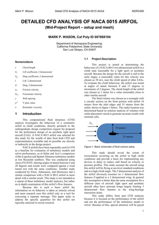
  • 1. Mark P. Wason Detail CFD Analysis of NACA 0015 Airfoil AERO406 1 DETAILED CFD ANALYSIS OF NACA 0015 AIRFOIL (Mid-Project Report – setup and mesh) MARK P. WASON, Cal Poly ID 007868194 Department of Aerospace Engineering, California Polytechnic State University San Luis Obispo, CA 93407 Nomenclature 𝑐 Chord length 𝐢𝑙 Lift coefficient, 2 dimensional 𝐢 𝑑 Drag coefficient, 2 dimensional 𝑙 Lift, 2 dimensional 𝑑 Drag, 2 dimensional π‘’βˆ— Friction velocity π‘ˆβˆž Freestream velocity y Wall spacing 𝑦+ Y-plus value 𝜈 Kinematic viscosity 1 Introduction This computational fluid dynamics (CFD) analysis investigates the behaviour of a symmetric airfoil in climb conditions, directly pertinent to the undergraduate design competition request for proposal for the preliminary design of an aerobatic light sport aircraft (LSA). A NACA 0015 airfoil was selected for this study for the wealth of data from both CFD and experimentation available and its possible use directly or indirectly in the design project. NACA airfoils have been repeatedly used in CFD as a baseline for evaluation of turbulence models and solver performance, as in Sahin and Acir’s comparison of the k-epsilon and Spalart Allmaras turbulence models at low Reynolds numbers. This was conducted using Ansys FLUENT, altering angles of attack between 2 and 20 degrees and results were compared against a wind tunnel test with the same conditions. Another study conducted by Eleni, Athanasios, and Dionissios did a similar comparison with a NACA 0012 airfoil in more detail with a similar result. This study is not intended as a repeat of these turbulence model analyses, but rather an in depth examination of this airfoil’s flow features. Because this is such a basic airfoil the information on its behavior is taken as entirely solved and most research uses this airfoil only as a tool for conveying a separate message. This paper seeks to address the specific quantities for this airfoil not typically analysed in recent research. 1.1 Project Description This project is aimed at determining the behaviour of a NACA 0015 two-dimensional airfoil in a climb state reasonable for a light sport or aerobatic aircraft. Because the design for the aircraft is still in the early stages, a reasonable value for this velocity was chosen as 30 m/s, near the climb speed of other LSAs. To evaluate the climb behaviour, the airfoil was tested at angles of attack between 8 and 15 degrees in increments of 2 degrees. The chord length of the airfoil was chosen as 1 meter for a value reasonably close to other similar aircraft. The fluid volume was chosen as a rectangle with a circular section on the front portion with airfoil 10 meters from the inlet edges and 35 meters from the outlet, shown in figure 1 below. The outlet location was determined based on solution analysis of volumes with outlet placement varied to generate accurate results with minimal cells. Figure 1. Basic schematic of fluid volume setup. This study should reveal the extent of recirculation occurring on the airfoil in high climb conditions and provide a basis for implementing any devices to delay or reduce stall based on velocity or pressure profiles. This study assumes the aircraft using this airfoil will be flying at sea level standard conditions and at a high climb angle. The 2 dimensional analysis of the airfoil obviously assumes no 3 dimensional flow features if applied to a 3 dimensional wing. In general this assumption is better than the same assumption for a different class of aircraft: light sport and aerobatic aircraft often have unswept wings largely limiting 3 dimensional flow features to the wing-fuselage interaction alone. This study differs from past CFD analyses because it is focused on the performance of the airfoil and not the performance of the turbulence model or solver. Because of this, special attention will be payed π‘ˆβˆž 10 meters 35 meters
  • 2. Mark P. Wason Detail CFD Analysis of NACA 0015 Airfoil AERO406 2 to the accuracy of the solution over turbulence model performance. 2 Test Conditions The Reynolds number for this test is around 2.1 million, so it is reasonable to expect largely turbulent flow over the airfoil. To model this in using Reynolds- averaged Navier-Stokes equations (RANS), the k- omega turbulence model is assumed for its mix of accurate modelling of near wall flows with the k-omega model and non-computationally expensive use of k- epsilon for outer flows. The k-omega model is particularly important for modelling of the turbulent transition and recirculation that will occur at higher angles of attack4 . This turbulent model is a starting point for future model comparisons and so can change based on accuracy of the model for this application. This study was conducted using Star-CCM+ CFD software created by CD-Adapco. Because the student version of Ansys has a limit on mesh size for creation and analysis, Star-CCM+ was the only commercial quality full CFD software package available. Results were determined to be converged when successive iterations did not change the mean value of residual terms significantly; this was done by visual inspection and samples of converged plots are shown in appendix B. Simulations were run in parallel on a windows 7 Enterprise operating system with local parallel processing using 8 cores with 16 gigabytes of RAM for increased speed. Solution runs typically took 1 to 2 hours to fully converge with around 400,000 cells. The final geometry is shown in figure 2 below, with flow moving from left to right from velocity inlet to pressure outlet. The inlet position in relation to the airfoil was chosen based on setups in other studies of similar airfoils and confirmed when no velocity change occurred outside a small region around the airfoil. The outlet position was determined based on a comparison of various outlet locations discussed further in section 2.1. Figure 2. Box and airfoil geometry setup. The flow was based on sea level climb conditions of a light sport aircraft, so gage pressure was set to zero for all boundaries and density at 1.225 kg/m^3. Alterations of angle of attack were done by changing the flow direction at the inlet to minimize meshing required and decrease processing time. 3 Grid description and refinement Initially a rectangular shaped bounding box was used to surround the airfoil with a hybrid mesh. The unstructured mesh was chosen because changing the angle of attack would require minimal additional effort and the prism layer would be able to achieve the desired y-plus value. The final stage of this mesh is shown in figure 3 below, where several volumetric controls have been applied to refine the areas around the wing and in the wake. Unfortunately, issues with the trailing edge caused errors where the prism layer met the unstructured mesh seen in figure 1a, and so was abandoned in favor of fully structured meshing. This original unstructured mesh also had 2 to 4 times the number of cells of the most accurate structured meshes, and so structured was pursued. Issues with convergence also hastened the switch, but these could likely have been resolved with fine manipulation of settings if a hybrid mesh was preferable. Figure 3. Final version of hybrid triangular and prism layer mesh. To facilitate structured meshing and reduce area required for meshing, a rectangular box with a circular front edge was chosen as the bounding box for the structured meshing. This is a similar shape to nearly every other 2 dimensional CFD airfoil analysis (eg. Sahin or Eleni), and allows for creation of an accurate structured mesh with minimal cells. Velocity Inlet Airfoil Pressure Outlet A) B) C)
  • 3. Mark P. Wason Detail CFD Analysis of NACA 0015 Airfoil AERO406 3 3.1 Solution Grid Independence A series of mesh alterations were evaluated to determine any influence on solution with simulations based on 0 degree angle of attack airfoil at a test speed of 1 m/s. This speed was chosen to match the Reynolds number of a study conducted by Sahin and Acir to compare basic results before moving to actual test conditions. The first comparison was conducted on the location of the outlet by changing the length of the rectangular section aft of the airfoil and tabulating coefficients of lift and drag. This alteration was conducted after successful simulation resulted in a trailing edge wake that stretched from the airfoil to the pressure outlet, and evaluation of the effect of this feature was necessary to proceed with simulation. The exact shape of the mesh aft of the airfoil changed slightly between tests, but the mesh upstream of the airfoil was the same. The solver used for this simulation was a realizable k-epsilon model to mimic the results obtained by Sahin and Acir. The full tabulated results of this study are shown in appendix C and the change in coefficient of drag is plotted below in figure 4. Based on the relatively large change from 25 meters to 35 meters in coefficient of drag (0.3 %) and the smaller change from 35 to 40 meters (0.09 %), it is reasonable to set the outlet at 35 meters from the airfoil. Even though this mesh was not particularly fine, it still agreed reasonably close with results from Sahin and Acir’s coefficient of drag of 0.028. Figure 4. Change in coefficient of drag based on pressure outlet location from trailing edge of airfoil. The mesh density was also modified to evaluate solution reliance; the results for this are shown in table 1. This was conducted at the test conditions of 30 m/s airspeed at sea level standard conditions using a k- omega SST turbulence model. The three meshes were made by first creating the finest resolution mesh (110,000 cells) and then reducing the cells by half and then half again to generate the other meshes. The three meshes had the same wall spacing with a y-plus value of approximately 1, low enough to capture the laminar sublayer and obtain highly accurate results6 . Because this airfoil is symmetric and at an angle of attack of 0 degrees, the coefficient of lift should theoretically be zero. To get a better value comparison, the change in drag coefficient will be examined since it will be non-zero and should vary more significantly. The grid convergence index was computed for the three simulations with the highest number of cells using Roache’s method of grid convergence indexing. With this method the ratio of grid convergence factors was found as 0.964, close enough to 1 to say the solutions are within the asymptotic range of convergence. Table 1 – Change in coefficients of lift and drag based on mesh density Cells Normalized Spacing CD 27,500 4 0.01299311 55,000 2 0.01028834 110,000 1 0.00991693 Using Richardson extrapolation, the projected value at a continuum grid spacing is shown in figure 5 along with the coefficients of drag from the simulations. Because the value changes very little (around 0.6%) between the lowest grid spacing and the projected value, it is reasonable to use the mesh with 110,000 cells over a finer mesh. Figure 5. Change in coefficient of drag based on mesh density. 3.2 Trailing Edge Geometry The typical airfoil trailing edge geometry using structured mesh is a sharp trailing edge instead of a rounded or blunt trailing edge. This generally makes the cell transition from the end of the airfoil to wake smoother with less acceleration from sharp angle changes. To investigate the difference in solution, a 0.02456 0.02458 0.0246 0.02462 0.02464 0.02466 0.02468 0.0247 0.02472 25 35 40 CoefficientofDrag Outlet from Airfoil (m) Outlet Location Comparison 8.00E-03 9.00E-03 1.00E-02 1.10E-02 1.20E-02 1.30E-02 1.40E-02 0 1 2 4 CoeffiicentofDrag Normalized Grid Spacing Mesh Density Comparison Projected Value
  • 4. Mark P. Wason Detail CFD Analysis of NACA 0015 Airfoil AERO406 4 geometry with a more rounded trailing edge and a geometry with a sharp trailing edge were compared, with the respective meshes shown in figure 6 a and b. These meshes were compared by running until the solution converged at the test conditions using a K- Omega SST turbulence model. Figure 6. Blunt (A) and sharp (B) trailing edge meshes for 8 degrees angle of attack. The accuracy of these trailing edge treatments were compared across all test angles of attack in figure 7 as a percent error of the converged solution. This percent error was calculated based on the oscillations occurring in the lift and drag values in the converged solution. Interestingly, the error is higher for the sharp trailing edge at lower angles of attack, but increases much more for the blunter trailing edge at higher angles. There is likely an error here that cannot be eliminated at these higher angles because flow separation creates an unsteady result from recirculation. The difference in the error however, is probably due to issues at the blunt trailing edge where cell skew is higher and the dramatic angle change forces the flow to accelerate more than it would realistically. Because of this, the sharp trailing edge geometry was chosen to proceed with simulation. It is worth noting that the blunt trailing edge does not have a lift or drag data point for 13 degrees angle of attack because of a meshing error. The mesh appeared adequate by visual inspection with comparable levels of maximum skew, but the error produced at this level was an order of magnitude higher than other values. It was left out to visualize the trends in the rest of the data better. Figure 7. Comparison of error in converged solution for lift (A) and drag (B) for sharp and blunt trailing edges. 3.3 Final Mesh The final mesh is shown in figure 8. The cells around the airfoil had a y-plus value of approximately 1, with no value above 2 for a converged simulation; this resulted in a wall spacing of 0.015 millimeters. This same spacing was carried through the trailing edge wake to the end of the bounding box. The mesh on the aft section of the airfoil also had a more refined mesh perpendicular to the boundary layer for refinement in possible separation zones. In order to generate the different angles, the airfoil was rotated while the fluid volume otherwise kept the same. Because each angle was a different geometry, it was necessary to create a new mesh for each part and so cell distributions were not completely consistent across the models. In an attempt to maintain consistency, each mesh was set up in a similar manner to the mesh for the 8-degree angle of attack mesh shown in figure 8 where the zones on the leading edge, center of airfoil, and trailing edge had similar cell density. Additionally, the wake region was setup as a straight section in each case from the trialing edge to the pressure 0 0.02 0.04 0.06 0.08 0.1 0.12 0.14 0.16 7 9 11 13 15 17 PercentError(%) Angle of Attack (degrees) Error in Lift Values Sharp Trailing Edge Blunt Trailing Edge 0 0.5 1 1.5 2 2.5 3 3.5 4 7 9 11 13 15 17 PercentError(%) Angle of Attack (degrees) Error in Drag Values A) B) A) B)
  • 5. Mark P. Wason Detail CFD Analysis of NACA 0015 Airfoil AERO406 5 outlet with cells finer at the trailing edge to show any vertical motion accurately. These regions give the leading edge enough refinement to accurately shape the airfoil curve as well as properly model the separation behavior. Figure 8. Final mesh at 8-degree angle of attack setup. 4 Turbulence Model Selection To better understand the solution reliance on turbulence model, four models were tested at 12-degrees angle of attack with the resulting coefficients of drag shown in figure 9. This angle was chosen since a model that performed well at this point would likely perform better in general for the rest of the angles than one that did not perform well here. Figure 9. Coefficient of drag based on turbulence model. Data from XFOIL shown for comparison. The coefficient of drag from XFOIL is also shown, providing a baseline for comparison. The turbulence models produced results reasonably close to each other, with SST, Wilcox and Spalart-Allamaras all falling within 1 standard deviation of the mean value of the 4 models. The realizable k-epsilon model falls within 2 standard deviations of the mean and is the furthest away from the XFOIL prediction. With these factors and the fact that the k-epsilon typically does not accurately predict behavior in adverse pressure gradients, it is reasonable to discount this model. Of the remaining models, the k-omega SST model was chosen for its robust approach to solution and accuracy in separated flow. The SST model uses the k- epsilon model for the freestream solution and the Wilcox k-omega model for the near wall treatment to account for the difficulty the Wilcox k-omega model can have solving for freestream conditions. Because the Wilcox k-omega model will solve for freestream, it makes sense that the results are similar to the SST turbulence model.4 5 Results and Discussion After using the k-omega SST model to evaluate the flow for each angle, the lift and drag coefficients for each angle were tabulated and compared to XFOIL, shown in figure 10 a and b. Error was calculated for each data point as in the trailing edge discussion by examining the variance in the converged simulation, but was not plotted here since it is too small to show up (see appendix C for full data tables). While the values from the CFD analysis do not agree completely with the numbers from XFOIL, both plots have the same shape as the XFOIL plots. Because the lift from CFD was lower at every value than XFOIL while drag was higher at every value, this seems to be a systematic offset. XFOIL and CFD use very different methods to calculate the flow, and since XFOIL is specifically constructed to analyse airfoils, it likely produces more accurate results. This is difficult to know for certain without wind tunnel testing, but because XFOIL is so well known and consistently close to past experiments, its results are probably more accurate. Because this difference exists, it is necessary to realize the possible error in this data before proceeding with any further analysis. 0.0200 0.0204 0.0215 0.0206 0.0146 0 0.005 0.01 0.015 0.02 0.025 CoeffiicientofDrag Turbulence Model Comparison A) B)
  • 6. Mark P. Wason Detail CFD Analysis of NACA 0015 Airfoil AERO406 6 Figure 10. Lift (A) and Drag (B) plotted against angle of attack for both XFOIL and CFD data. To find the separation zones on this airfoil, the velocity in the x-direction was plotted and the separation point was taken as the first location where it became negative on the upper surface of the airfoil. This is shown for the 15-degree case in figure 11 below where the colored spaces represent all area of negative x- velocity. Figure 11. Negative x-velocities shown in color depicting separation regions. This was compared against XFOIL results for the same case and shown in table 2 below. Looking at the two, CFD predicts separation earlier than XFOIL, by as much as 6% of the chord for the 15-degree test. Again, the only way to truly validate this would be with a wind tunnel experiment. Unfortunately, as this is not in the scope of the project, the XFOIL results are taken as closer to correct than the CFD. The CFD results are still useful as something of a conservative estimate of the separation behaviour until this can be validated. Table 2 – Change in stall point from XFOIL and CFD based on angle of attack. Stall Point (% of chord) Angle of Attack XFOIL CFD 8 100 100 9 100 100 10 100 100 11 100 100 12 100 100 13 100 95.6 14 97 92 15 93 86.5 At these conditions, neither CFD nor XFOIL predicted a dramatic stall condition, and so no devices to reduce stall would be required for this airfoil to achieve adequate performance at these conditions. Even if the more conservative separation numbers from CFD are used to determine the separation point, this airfoil still maintains adequate performance. A final plot of lift to drag ratio was made for both XFOIL and CFD data, and is shown in figure 12. It is clear that while the values are different between the two data sets, the highest ratio is predicted in the same location at 10 degrees. While this prediction has not been truly validated, the consistency in predictions leads to the conclusion that the actual value is close to this prediction. This is valuable information for proceeding with integration of this airfoil into an aircraft. 0.7 0.8 0.9 1 1.1 1.2 1.3 1.4 1.5 1.6 7 9 11 13 15 17 CoefficientofLift Angle of Attack (degrees) Lift vs Angle of Attack CFD XFoil 0 0.005 0.01 0.015 0.02 0.025 0.03 0.035 7 9 11 13 15 17 CoeffiicientofDrag Angle of Attack (degrees) Drag vs Angle of Attack A) B) Separation point A) B) C)
  • 7. Mark P. Wason Detail CFD Analysis of NACA 0015 Airfoil AERO406 7 Figure 12. Lift to drag ratio plotted for XFOIL and CFD data. 6 Conclusions The mesh for this simulation was created after a series of solution dependence studies determined the effects of various parameters. From this it was concluded that the outlet must be placed 35 meters from the airfoil and that 110,000 cells was sufficient to achieve grid independence. Additionally, the geometry of the trailing edge was set as a point instead of a round or blunt edge to reduce solution uncertainty and improve mesh quality. When comparing to XFOIL results, the CFD analysis predicted consistently lower lift and higher drag, and must be analysed with an experimental test to determine the validity of the solution. Since XFOIL has been validated in similar tests, it is likely more accurate than the CFD analysis but may not be totally correct. This could be due to a number of factors, but because XFOIL and CFD are so different in formulation it is difficult to pinpoint exactly what causes the discrepancy in values. If the results from this study were to be taken to another level of analysis, a 3 dimensional evaluation of this airfoil’s performance on a specific wing in the application of the aerobatic aircraft would be helpful. Since this analysis would be much more specific than the two dimensional study here, it would be best if the preliminary design of the aircraft wing was completed to get the best results from the simulation. With a single specific simulation, this could also be verified against a wind tunnel test to generate an extremely accurate result for wing performance in climb conditions. Another approach for further analysis would be modifying the parameters of the aircraft in a series of simulations to examine effect of twist, sweep, wing placement, and taper. These would need to be much less exact than the specific simulations mentioned previously in order to be completed in a similar amount of time, and so would be less accurate and not likely to be validated. In this case the simulation would be an aspect of design and so the results would only need to be rough to get the required information. 40 50 60 70 80 90 100 7 9 11 13 15 17 LifttoDragRatio Angle of Attack (degrees) Lift to Drag CFD XFoil
  • 8. Mark P. Wason Detail CFD Analysis of NACA 0015 Airfoil AERO406 8 Appendices A. Miscellaneous equations Coefficient of lift: 𝐢𝑙 = 𝑙 1 2 πœŒπ‘ˆβˆž 2 𝑐 Coefficient of drag: 𝐢 𝑑 = 𝑑 1 2 πœŒπ‘ˆβˆž0 2 𝑐 Y-plus: 𝑦+ = π‘’βˆ— 𝑦 𝜈 B. Sample Residual Plot C. Tabulated Data Coefficients of lift and drag based on outlet position Outlet Position (m) Cl Cd Cells 25 -3.2221857691183686E-4 0.024700382724404335 537500 35 4.628599e-04 2.463374e-02 637500 40 7.594945e-05 2.461226e-02 737500
  • 9. Mark P. Wason Detail CFD Analysis of NACA 0015 Airfoil AERO406 9 Coefficients of lift and drag calculated with CFD. Angle of Attack Coefficient of Lift Coefficient of Drag Value % Error Value % Error 8 0.827895 0.000603941 0.014851 0.000673337 9 0.933387 0.000374979 0.015149 0.002640508 10 1.0255 0.000195027 0.016599 0.003614719 11 1.118605 0.00759875 0.018105 0.091134542 12 1.20347 0.010802097 0.020039 0.143222149 13 1.28398 0.035047275 0.022349 0.49666874 14 1.35532 0.030988992 0.025122 0.43587988 15 1.41441 0.028987352 0.028776 0.380879568 References [1] Eleni, Douvi C. "Evaluation of the Turbulence Models for the Simulation of the Flow over a National Advisory Committee for Aeronautics (NACA) 0012 Airfoil." J. Mech. Eng. Res. Journal of Mechanical Engineering Research 4.3 (2012): 100-11. Web. 8 Nov. 2015. [2] "Examining Spatial (Grid) Convergence." Examining Spatial (Grid) Convergence. NASA, 17 July 2008. Web. 09 Nov. 2015. [3] Jacobs, Eastman N., Kenneth E. Ward, and Robert M. Pinkerton. "The Characteristics of 78 Related Airfoil Sections from Tests in the Variable-Density Wind Tunnel." (n.d.): n. pag. NASA. Web. 8 Nov. 2015. [4] Menter, F. R., M. Kuntz, and R. Langtry. (n.d.): n. pag. Software Development Department, ANSYS - CFX. Web. 8 Nov. 2015. [5] Şahin, Izzet, and Adem Acir. "Numerical and Experimental Investigations of Lift and Drag Performances of NACA 0015 Wind Turbine Airfoil." International Journal of Materials, Mechanics and Manufacturing IJMMM 3.1 (2015): 22-25. Web. 8 Nov. 2015. [6] "Tips & Tricks: Estimating the First Cell Height for Correct Y+." Computational Fluid Dynamics CFD Blog LEAP Australia New Zealand. N.p., n.d. Web. 09 Nov. 2015.