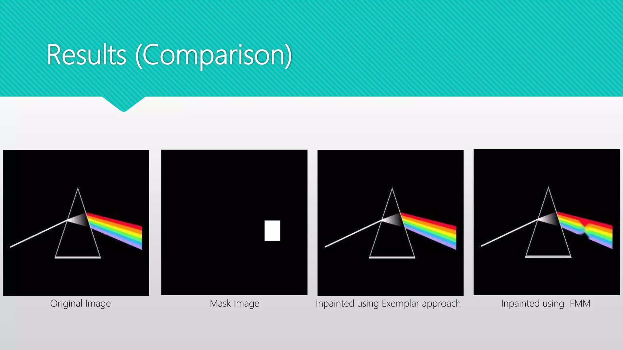
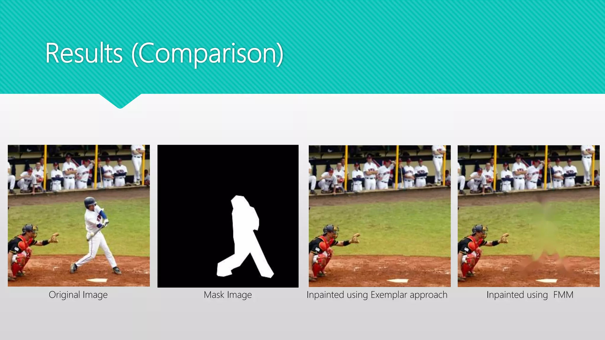
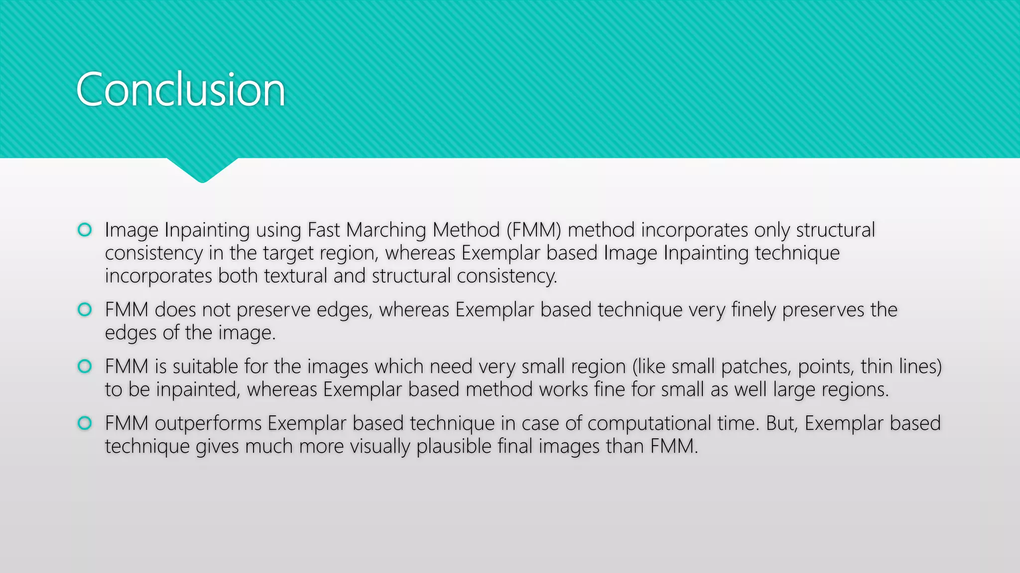
This document compares two image inpainting algorithms: the Fast Marching Method (FMM) and exemplar-based image inpainting. FMM uses structural consistency to fill damaged regions, while exemplar-based uses both structural and textural consistency. FMM is faster but does not preserve edges as well as exemplar-based. Exemplar-based works for both small and large regions but is slower. Both algorithms were tested on photos for tasks like removing objects or adding effects. Exemplar-based was better for large regions and edge preservation, while FMM was better for speed and small regions.

1. Comparative Analysis of Image
Inpainting Algorithms.
Supervised by : Submitted by:
Dr. Ranjana Vyas Lavesh Kaushik (IIT2013062)
Manav Sharma (IIT2013173)

2. Outline
 Introduction
 Motivation
 Problem Definition and Statement
 Methodology
 Results
 Conclusion
 References

3. Introduction
 Image Inpainting is technique of reconstructing damaged images by filling in the lost data of the
image.
 Motive is not to reconstruct the original image (because the information is lost, there is no way to
recover that), but to recover in visually plausible manner such that it looks legitimate to the
human eye.
 Three groups of 2D image inpainting algorithms :
• Structural inpainting.
• Textural inpainting.
• Combined Structural and Textural inpainting.

4. Motivation
 There are many old photos that get damaged with unwanted spots and lines.
 Also we have need to remove unwanted objects from some images.
 Moreover, there can be a lot of text in the image that is required to be removed.
 So, basically there is requirement to fill the lost or refill the unwanted information from the known
information (i.e. background).
 This in turn can also be used to add special effects to images.

5. Problem Statement and Definition
 Implementing 2 Image Inpainting algorithms namely,
1. Image Inpainting Technique Based on the Fast Marching Method.
2. Exemplar-Based Image Inpainting.
 Both the algorithms were then tested on many different images to understand which algorithm
outperforms other and when to use which algorithm.

6. Methodology (Fast Marching Method)
Mathematical Model:
• p: point to be inpainted
• Ω: region to be inpainted
• dΩ: boundary of the
region Ω to be inpainted
• Bε(p): ε- ball of the known image
around some unknown point p

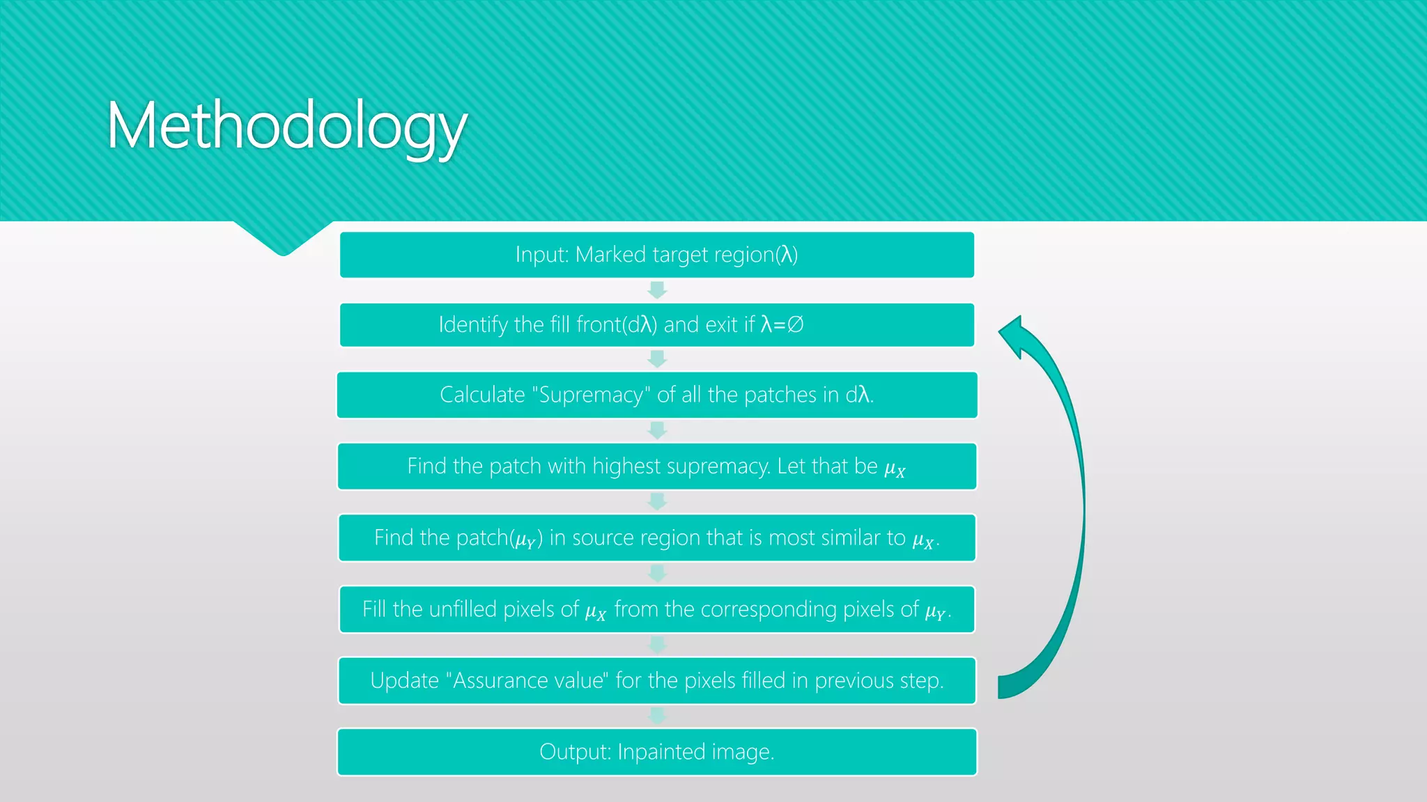
7. Methodology
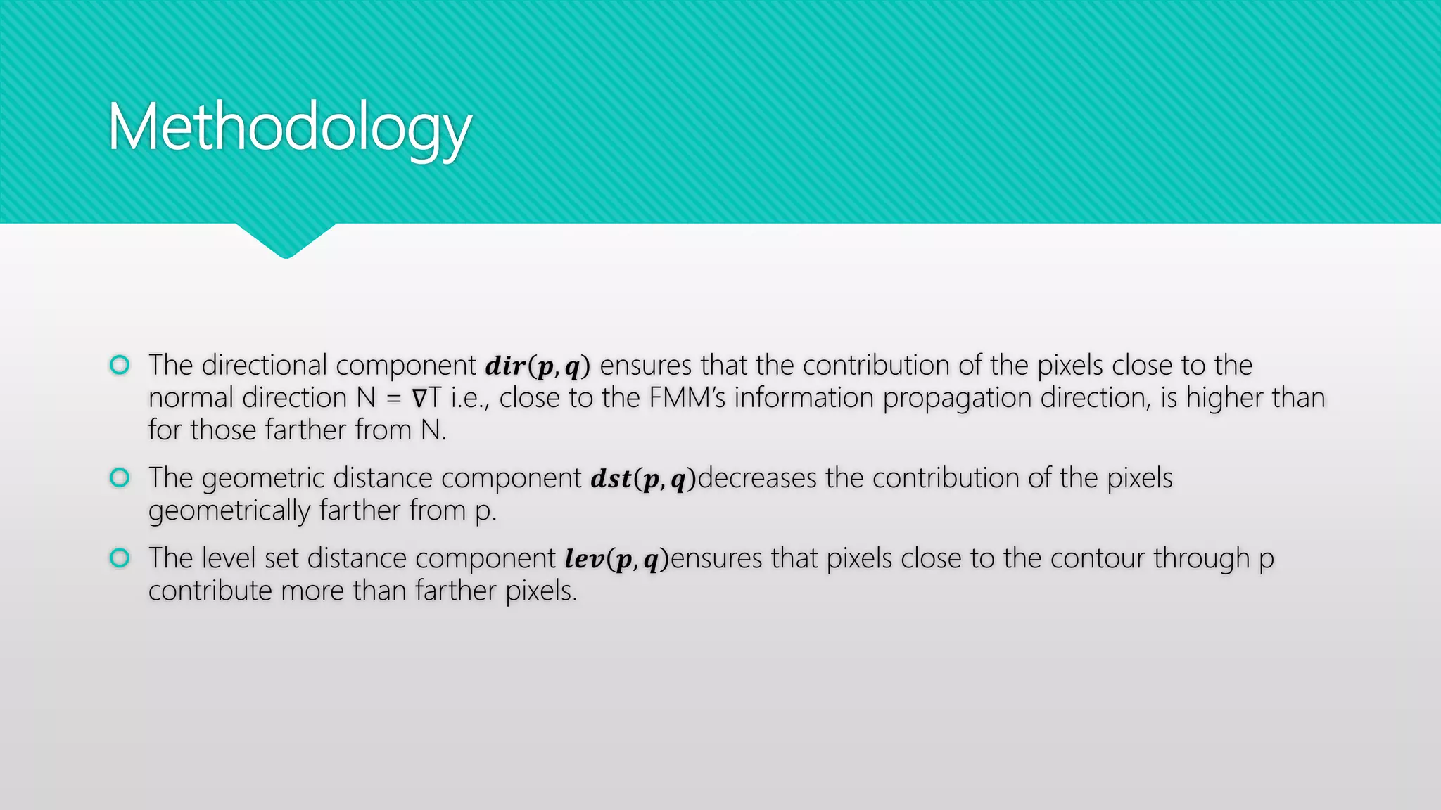
 For ε small enough, we consider a first order approximation Iq(p) of the image in point p, given
the image I(q) and gradient ∇I(q) values of point q :
𝐼 𝑞 𝑝 = 𝐼 𝑞 + 𝛻𝐼 𝑞 ∗ (𝑝 − 𝑞) (Eqn. 1)
 Next, we inpaint point p as a function of all points q in Bε(p) by summing theestimates of all
points q, weighted by a normalized weighting function w(p, q):
𝐼 𝑝 =
𝑞∈ 𝐵∈(𝑝) 𝑤 𝑝,𝑞 [𝐼 𝑞 + 𝛻𝐼 𝑞 𝑝−𝑞 ]
𝑞∈ 𝐵∈(𝑝) 𝑤 𝑝,𝑞
(Eqn. 2)

8. Flow Chart:
Input: Marked target region(Ω)
Find boundary of target region(dΩ)
Store some known neighboring points of the target region(that will be further used to propagate
color information inside target region).
Initialise Travel Time of all points in boundary of target region as 0 and push them in min heap.
Pop out a point p from heap and Inpaint it. Consider it to be known now.
Take neighboring points of p that are in target region, update their travel time and push them to
heap.
If heap is not empty, continue the loop.
Output: Inpainted image.

9. Methodology
Inpainting 1 point:
We iterate over the KNOWN points in the neighborhood Bε of the current point (i,j) and compute I(i,
j) following Equation 2. The image gradient ∇I is estimated by central differences.
We design 𝑤 𝑝, 𝑞 = 𝑑𝑖𝑟 𝑝, 𝑞 . 𝑑𝑠𝑡 𝑝, 𝑞 . 𝑙𝑒𝑣 𝑝, 𝑞
as a product of three factors:
 𝑑𝑖𝑟 𝑝, 𝑞 =
𝑝−𝑞
| 𝑝−𝑞 |
∗ 𝑁(𝑝)
 𝑑𝑠𝑡 𝑝, 𝑞 =
𝑑0
2
| 𝑝−𝑞 |2
 𝑙𝑒𝑣 𝑝, 𝑞 =
𝑇0
1+|𝑇 𝑝 −𝑇 𝑞 |

10. Methodology
 The directional component 𝒅𝒊𝒓 𝒑, 𝒒 ensures that the contribution of the pixels close to the
normal direction N = ∇T i.e., close to the FMM’s information propagation direction, is higher than
for those farther from N.
 The geometric distance component 𝒅𝒔𝒕 𝒑, 𝒒 decreases the contribution of the pixels
geometrically farther from p.
 The level set distance component 𝒍𝒆𝒗 𝒑, 𝒒 ensures that pixels close to the contour through p
contribute more than farther pixels.

11. Methodology (Exemplar Based Image
Inpainting)
Mathematical Model:
 𝜌: Source region.
 𝜆: Target region.
 𝑑𝜆: Contour.
 𝜇 𝑥: Patch centered on point x.
 n: Unit vector perpendicular to 𝑑𝜆 at point x.
 G: Gradient of point x.

12. Methodology
Input: Marked target region(λ)
Identify the fill front(dλ) and exit if λ=Ø
Calculate "Supremacy" of all the patches in dλ.
Find the patch with highest supremacy. Let that be 𝜇 𝑋
Find the patch(𝜇 𝑌) in source region that is most similar to 𝜇 𝑋.
Fill the unfilled pixels of 𝜇 𝑋 from the corresponding pixels of 𝜇 𝑌.
Update "Assurance value" for the pixels filled in previous step.
Output: Inpainted image.

13. Results(FMM)
 Repairing Photographs

14. Results(FMM)
 Remove unwanted objects

15. Results(FMM)
 Special Effects

16. Results(Exemplary Based Technique)
 Preserving Edges

17. Results(Exemplar Based Technique)
 Large Object Removal

18. Results(Exemplary Based Technique)
 Removing Multiple Objects

19. Results (Comparison)
Original Image Mask Image Inpainted using Exemplar approach Inpainted using FMM

20. Results (Comparison)
Original Image Mask Image Inpainted using Exemplar approach Inpainted using FMM

21. Conclusion
 Image Inpainting using Fast Marching Method (FMM) method incorporates only structural
consistency in the target region, whereas Exemplar based Image Inpainting technique
incorporates both textural and structural consistency.
 FMM does not preserve edges, whereas Exemplar based technique very finely preserves the
edges of the image.
 FMM is suitable for the images which need very small region (like small patches, points, thin lines)
to be inpainted, whereas Exemplar based method works fine for small as well large regions.
 FMM outperforms Exemplar based technique in case of computational time. But, Exemplar based
technique gives much more visually plausible final images than FMM.

22. References
 Alexandru Telea (2006), “An Image Inpainting Technique Based on the Fast Marching Method”: Journal
of Graphic Tools UMCG Research, Vol. 9, No. 1.
 Shailendra Mishra, Ankit Prajapati and Pritika Patel (2012), “Review of Different Inpainting Algorithms”:
International Journal of Computer Applications, Vol. 9, No. 18.
 Antonio Criminisi, Patrick Pérez, and Kentaro Toyama (2004), “Region Filling and Object Removal by
Exemplar-Based Image Inpainting”: IEEE TRANSACTIONS ON IMAGE PROCESSING, Vol. 13, No. 9.
 Manuel M. Oliveira, Brian Bowen, Richard McKenna and Yu-Sung Chang (2001), “Fast Digital Image
Inpainting”: International Conference on Visualization, Imaging and Image Processing (VIIP 2001).
 P. Sengottuvelan, E. Balamurugan (2011), “Analysis of Exemplar Based Image Inpainting Algorithms”:
European Journal of Scientific Research, Vol. 60, No. 3.

23. THANK YOU