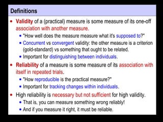
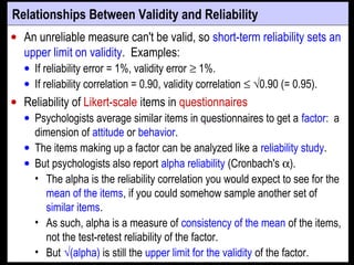
- Reliability is a measure of reproducibility of a test when repeated, quantifying random error. Validity is how well a test measures what it intends to, requiring comparison to a criterion. - Reliability is typically quantified by the typical error or intraclass correlation. Validity uses correlation and error of estimate from regression of the test on a criterion. - Both reliability and validity should be high for a test to accurately track small individual changes over time and distinguish individuals. Ideal values are >0.96 for reliability and validity correlations and typical/estimate errors <20% of between-subject standard deviation.

1. Validity and Reliability
Will G Hopkins (will@clear.net.nz)
Sport and Recreation
AUT University
• This slideshow is a shortened version of the slideshow in:
• Hopkins WG (2004). How to interpret changes in an athletic
performance test. Sportscience 8, 1-7. See link at sportsci.org.
• Other resources:
• Hopkins WG (2000). Measures of reliability in sports medicine and
science. Sports Medicine 30, 1-15.
• Paton CD, Hopkins WG (2001). Tests of cycling performance. Sports
Medicine 31, 489-496.
• Hopkins WG (2010). A Socratic dialogue on comparison of measures.
Sportscience 14, 15-21. See link at sportsci.org.
• My spreadsheets for analysis of validity and reliability. Also minor
articles. See links at sportsci.org.

2. Definitions
• Validity of a (practical) measure is some measure of its one-off
association with another measure.
• "How well does the measure measure what it's supposed to?"
• Concurrent vs convergent validity: the other measure is a criterion
(gold-standard) vs something that ought to be related.
• Important for distinguishing between individuals.
• Reliability of a measure is some measure of its association with
itself in repeated trials.
• "How reproducible is the practical measure?"
• Important for tracking changes within individuals.
• High reliability is necessary but not sufficient for high validity.
• That is, you can measure something wrong reliably!
• And if you measure it right, it must be reliable.

3. • We can often assume a measure is valid in itself…
• …especially when there is no obvious criterion measure.
• Examples from sport: tests of agility, repeated sprints, flexibility.
• If relationship with a criterion is an issue, usual approach is to assay
practical and criterion measures in 100 or so subjects.
• Fitting a line or curve provides
a calibration equation, the error of the
estimate, and a correlation coefficient.
• These apply only to subjects similar
to those in the validity study.
• Preferable to Bland-Altman analysis.
• Limits of agreement (= ±1.96× SD
of difference scores) do not allow proper assessment of error.
• B-A plot of difference vs mean scores usually indicates a systematic
offset error (“proportional bias”) when in reality there is none.
Practical body fat (%BM)Practical body fat (%BM)
CriterionCriterion
body fatbody fat
(%BM)(%BM)
Validity
r = 0.80

4. • Beware of units of measurement that lead to spurious high correlations.
• Example: a practical measure of body fat in kg might have a high
correlation with the criterion, but…
• Express fat as % of body mass and correlation = 0!
• So the measure provides no useful information.
• For many measures, use log transformation to get uniformity of error of
the estimate over the range of subjects.
• Check for non-uniformity in a plot of residuals vs predicteds.
• Use the appropriate back-transformation to express the error as a
coefficient of variation (percent of predicted value).
• The error of the estimate is the "noise" in the prediction.
• Ideally, noise < “signal”.
• The signal is the smallest important difference between subjects.
• Default = 0.20 of between-subject standard deviation (Cohen).
• But r2
= "variance explained" = (SD2
-error2
)/SD2
.
• So if noise < signal, error < 0.20*SD.
• It follows that ideally r > 0.98! Much higher than people realize.

5. • Uses of validity
• “Calibration” of a practical measure.
• The regression line between the criterion and the practical measure
converts the practical into an unbiased estimate of the criterion.
• The standard error of the estimate is the random error in the
calibrated value.
• Adjustment of effects in studies involving the practical measure
(“correction for attenuation”).
• If the effect is a correlation, it is attenuated by a factor equal to the
validity correlation.
• If the effect is slope or a difference or change in the mean, it is
attenuated by a factor equal to the square of the validity correlation.
• BEWARE: the calibration and adjustments apply only to subjects
drawn from the population used for the validity study.
• Otherwise the validity statistics themselves need adjustment.
• I have developed as yet unpublished spreadsheets for this purpose.

6. Reliability
• Reliability is reproducibility of a measurement
if or when you repeat the measurement.
• It's important for practitioners…
• because you need good reproducibility to monitor small but
practically important changes in an individual subject.
• It's crucial for researchers…
• because you need good reproducibility to quantify such changes in
controlled trials with samples of reasonable size.

7. • How do we quantify reliability?
Easy to understand for one subject tested many times:
Chris
Subject
76
Trial 2
72
Trial 1
74
Trial 3
79
Trial 4
79
Trial 5
77
Trial 6
76.2 ± 2.8
Mean ± SD
• The 2.8 is the standard error of measurement.
• I call it the typical error, because it's the typical difference between
the subject's true value and the observed values.
• It's the random error or “noise” in our assessment of clients and in
our experimental studies.
• Strictly, this standard deviation of a subject's values is the
total error of measurement rather than the standard or typical error.
• It’s inflated by any "systematic" changes, for example a learning
effect between Trial 1 and Trial 2.
• Avoid this way of calculating the typical error.

8. • We usually measure reliability with many subjects tested
a few times:
Chris
Subject
7672
Trial 2Trial 1
4
Trial 2-1
• The 3.4 divided by √2 is the typical error.
• The 3.4 multiplied by ±1.96 are the limits of agreement.
• The 2.6 is the change in the mean.
• This way of calculating the typical error keeps it separate from the
change in the mean between trials.
Jo 5853 5
Kelly 6060
Pat 8284
Sam 7367
0
-2
6
Mean ± SD: 2.6 ± 3.4

9. • And we can define retest correlations:
Pearson (for two trials) and intraclass (two or more trials).
• These are calculated differently but have practically the same
values.
• The typical error is more
useful than the correlation
coefficient for assessing
changes in a subject.
Trial 1
50
70
90
50 70 90
Trial 2
Intraclass r = 0.95
Pearson r = 0.95

10. • Uses of reliability: monitoring change in an individual…
• Think about ± the typical error as the noise or uncertainty in the
change you have just measured.
• You want to be confident about measuring the signal (smallest
worthwhile change), say 0.5%.
• Example: you observe a change of 1%, and the typical error is 2%.
• So your uncertainty in the change is 1 ± 2%, or -1% to 3%.
• So the change could be harmful through quite beneficial.
• So you can’t be confident about the observed beneficial change.
• But if you observe a change of 1%, and the typical error is only
0.5%, your uncertainty in the change is 1 ± 0.5%, or 0.5% to 1.5%.
• So you can be reasonably confident you have a small but
worthwhile change.
• Conclusion: ideally, you want typical error < smallest change.
• If typical error > smallest change, try to find a better test.
• Or repeat the test several times and average the scores to
reduce the noise. (Four tests halves the noise.)

11. • Importance of time between trials…
• When testing individuals, you need to know the noise of the test
determined in a reliability study with a time between trials short
enough for the subjects not to have changed substantially.
• Exception: to assess change due specifically to, say, a 4-
week intervention, you will need to know the 4-week noise.
• For estimating sample sizes for research, you need to know the
noise of the test with the same time between trials as in your
intended study.
• Beware: noise may be even higher in the study (and therefore
sample size will need to be larger) because of individual
responses to the intervention.
– Individual responses can be estimated from the difference in
noise between the intervention and control groups.

12. • More on noise…
• As with validity, use log transformation to get uniformity of error
over the range of subjects for some measures.
• Check for non-uniformity in a plot of residuals vs predicteds or
change scores vs means.
• Use the appropriate back-transformation to express the error as
a coefficient of variation (percent of subject's mean value).
• Ideally, noise < signal, and if signal = 0.20×SD, we can work out the
reliability correlation:
• Intraclass r = (SD2
-error2
)/SD2
– Validity equation is r2
= (SD2
-error2
)/SD2
.
• But want noise < signal; that is, error < 0.20×SD.
• So ideally r > 0.96! Again, much higher than people realize.

13. • Uses of reliability: estimating sample size for studies with repeated
measurement…
• In particular, changes in the mean in a crossover and differences in
the changes in a parallel-groups controlled trial.
• My sample-size spreadsheet is set up for using the typical error, but
you can convert a correlation to a typical error via a formula shown in
the spreadsheet.
• For typical error = smallest important effect, sample size = 10 for a
crossover and 24 (12+12) for a parallel-groups trial, using my method
of acceptable uncertainty in the outcome. For the traditional
approach, sample size is ~3x larger.
• For each doubling of the typical error, sample size increases by 4x.

14. Relationships Between Validity and Reliability
• An unreliable measure can't be valid, so short-term reliability sets an
upper limit on validity. Examples:
• If reliability error = 1%, validity error ≥ 1%.
• If reliability correlation = 0.90, validity correlation ≤ √0.90 (= 0.95).
• Reliability of Likert-scale items in questionnaires
• Psychologists average similar items in questionnaires to get a factor: a
dimension of attitude or behavior.
• The items making up a factor can be analyzed like a reliability study.
• But psychologists also report alpha reliability (Cronbach's α).
• The alpha is the reliability correlation you would expect to see for the
mean of the items, if you could somehow sample another set of
similar items.
• As such, alpha is a measure of consistency of the mean of the items,
not the test-retest reliability of the factor.
• But √(alpha) is still the upper limit for the validity of the factor.