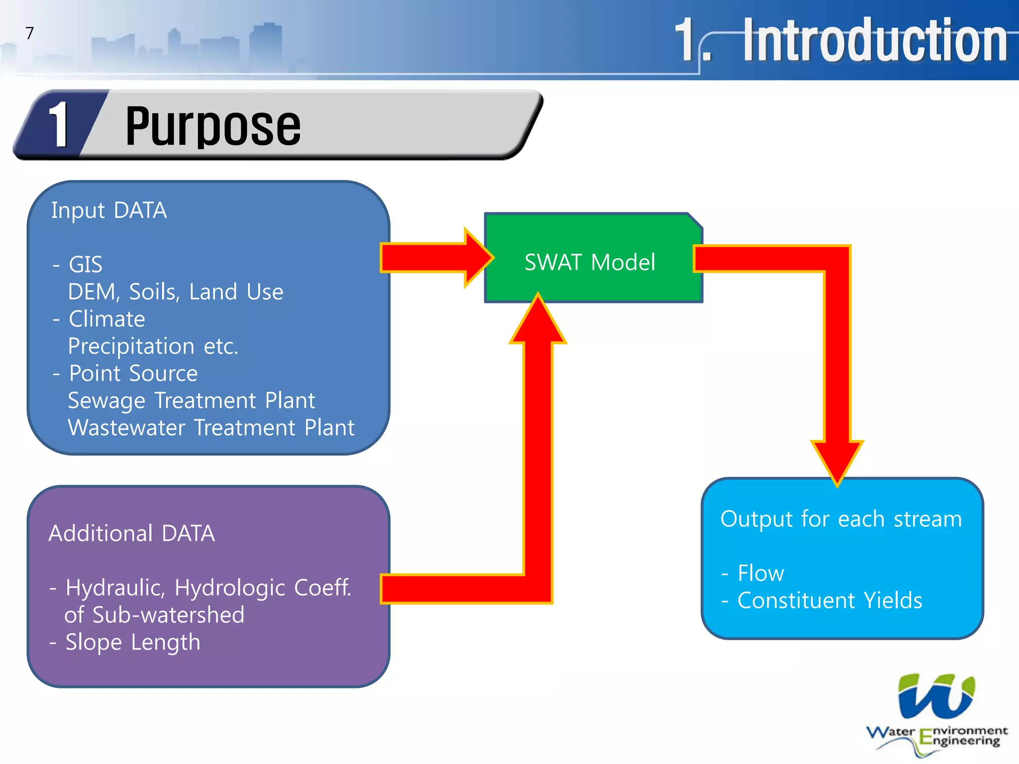
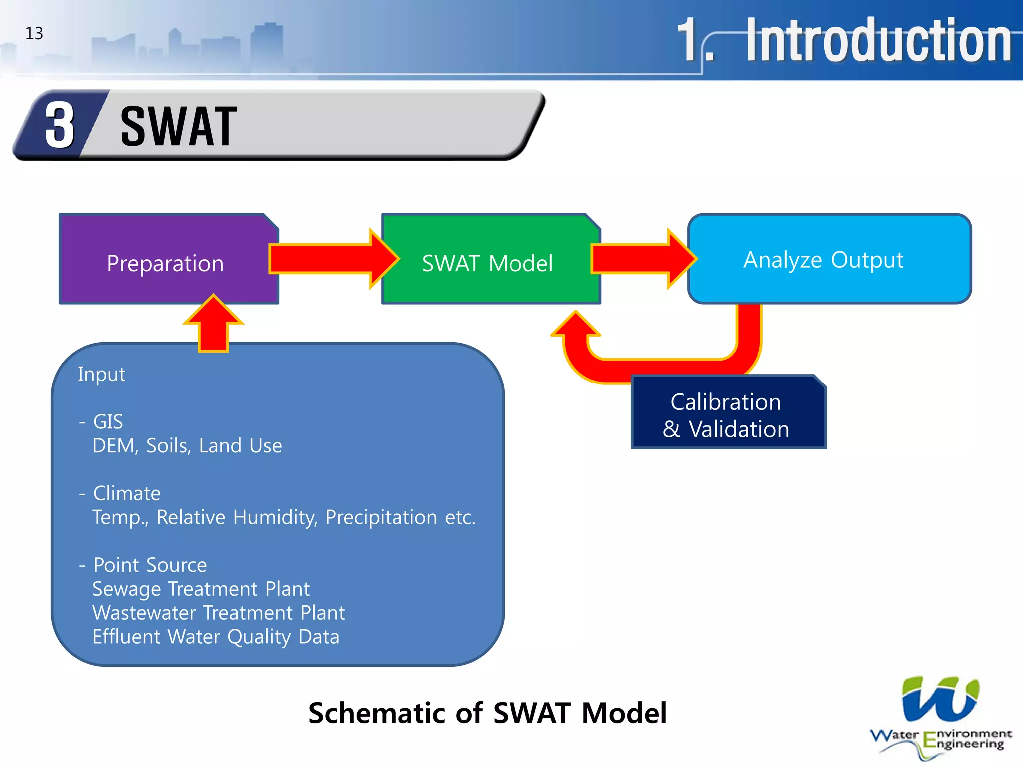
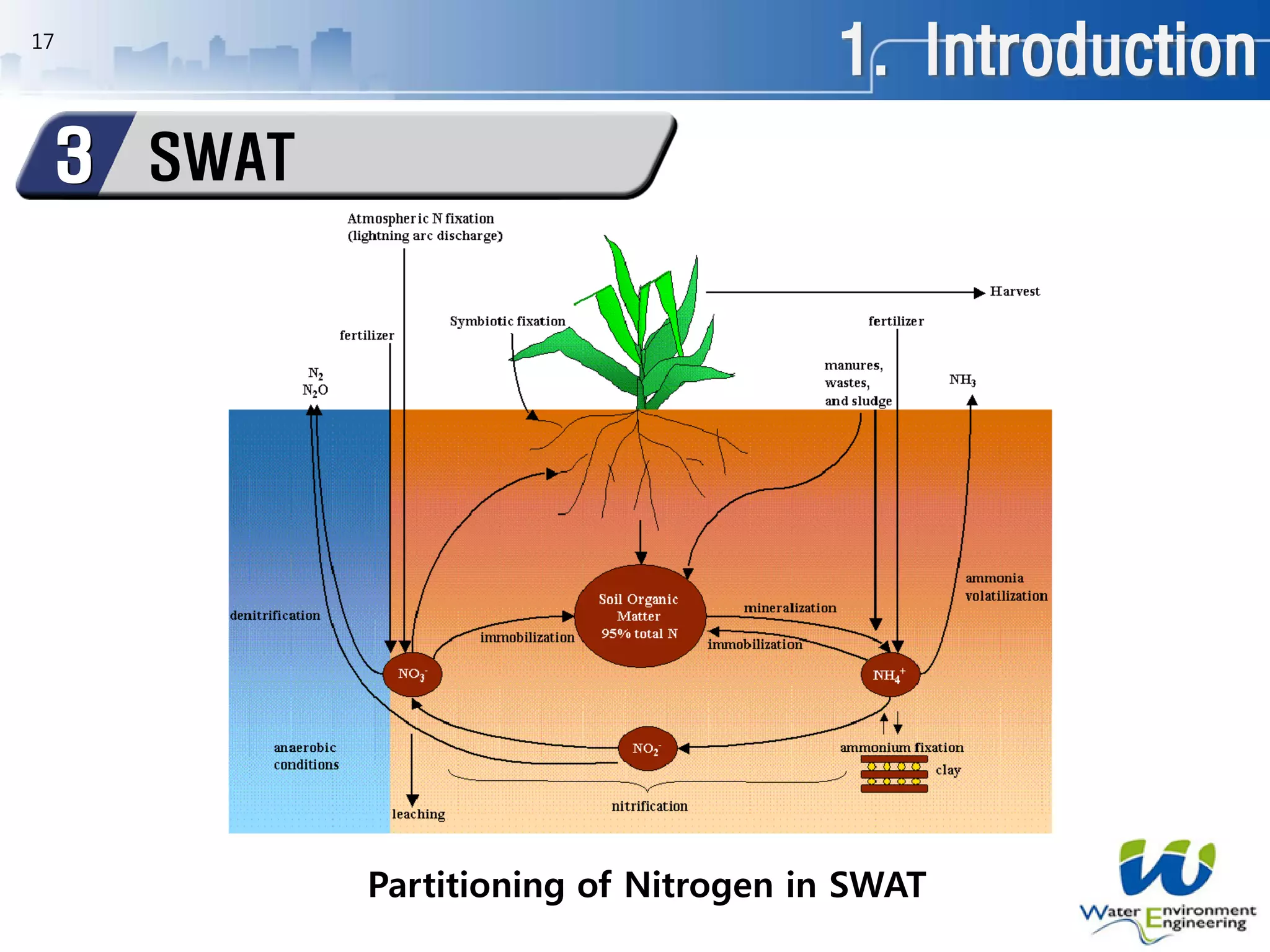
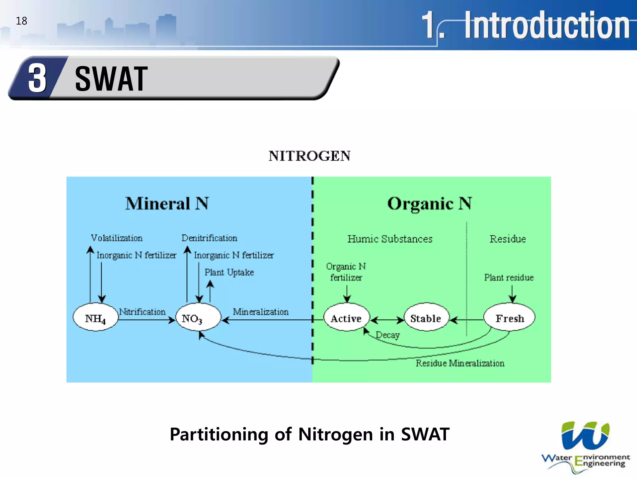
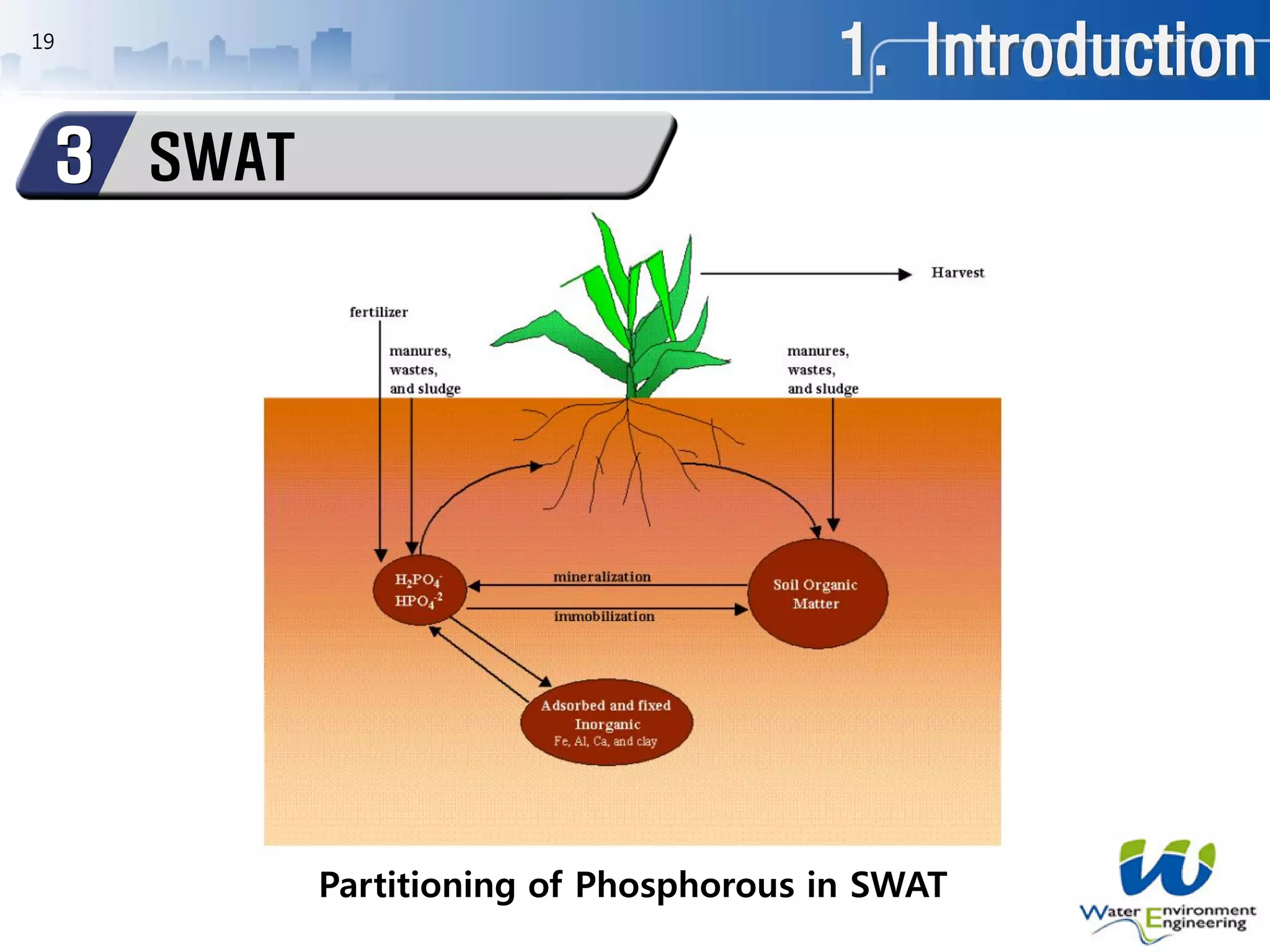
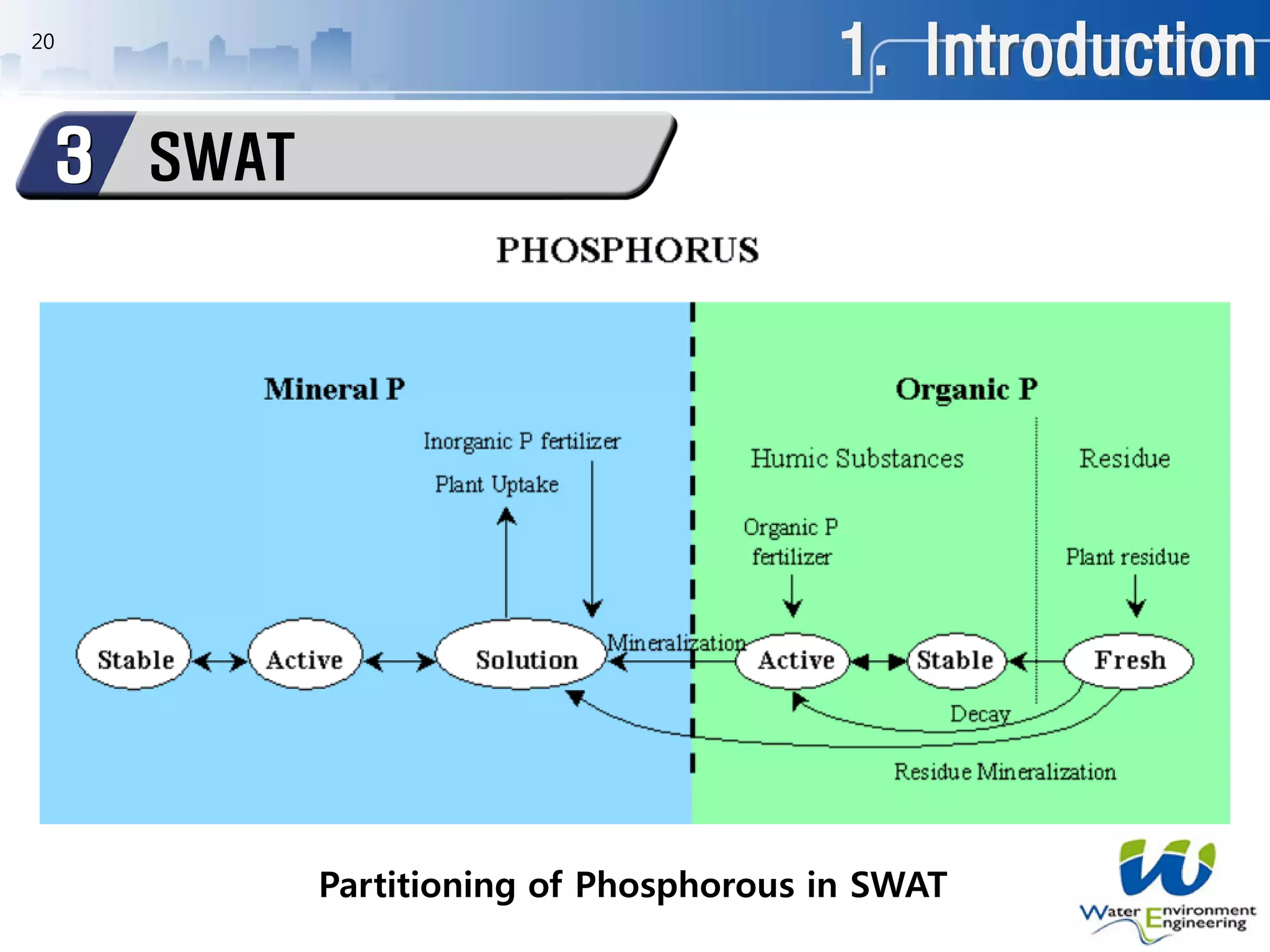
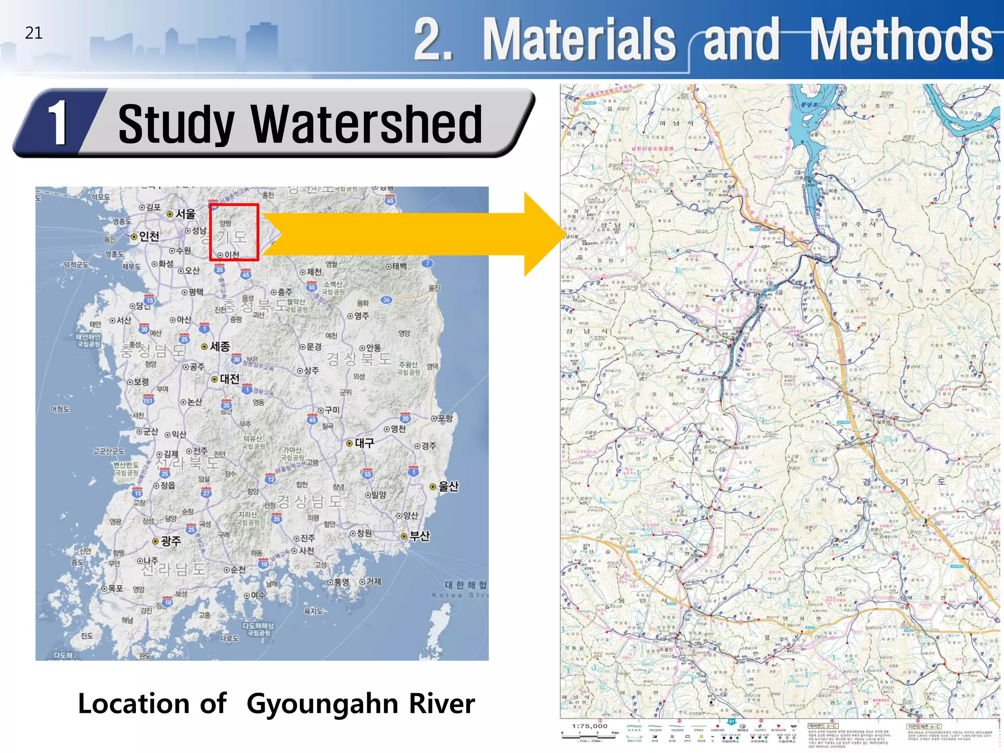
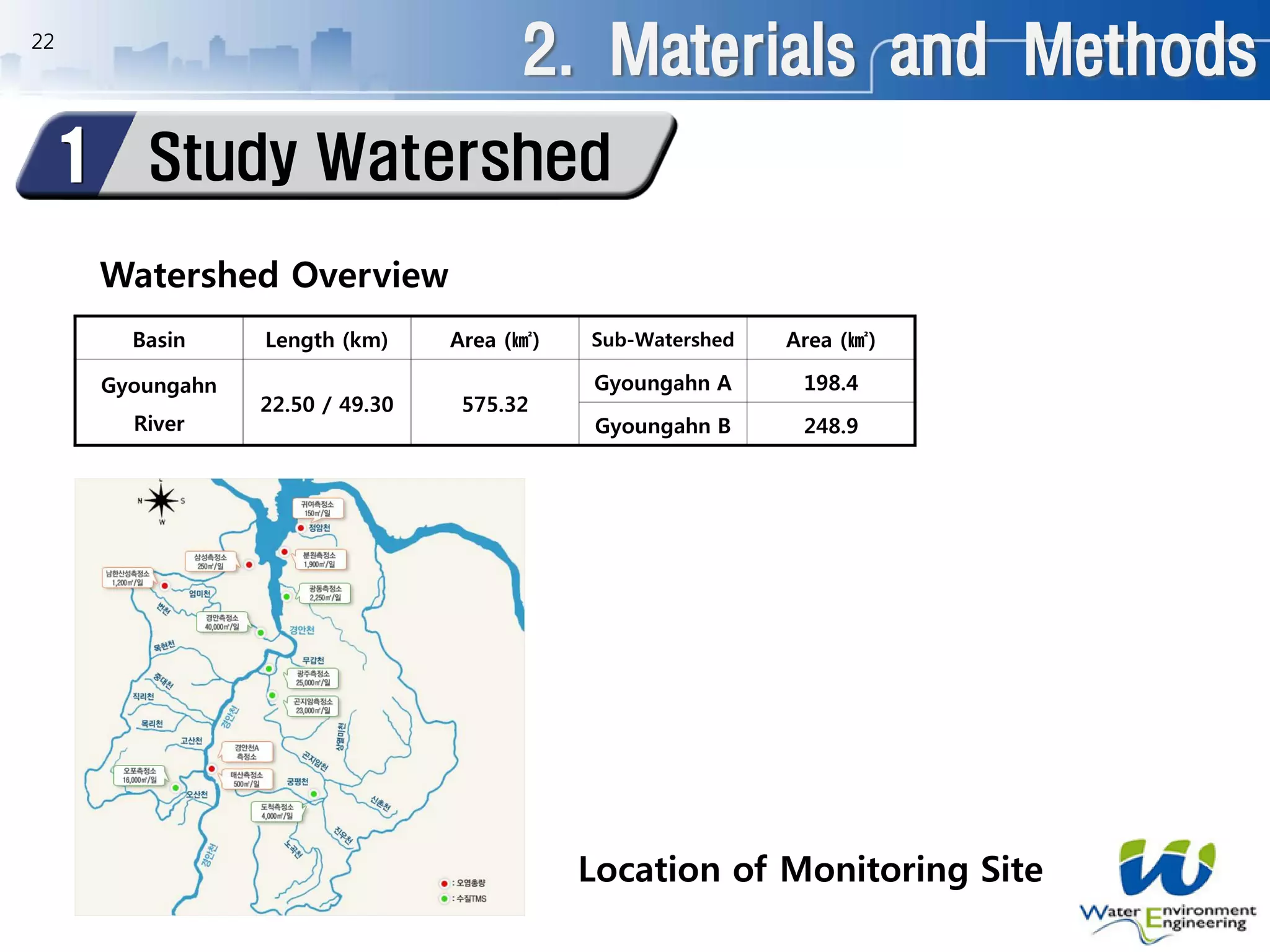
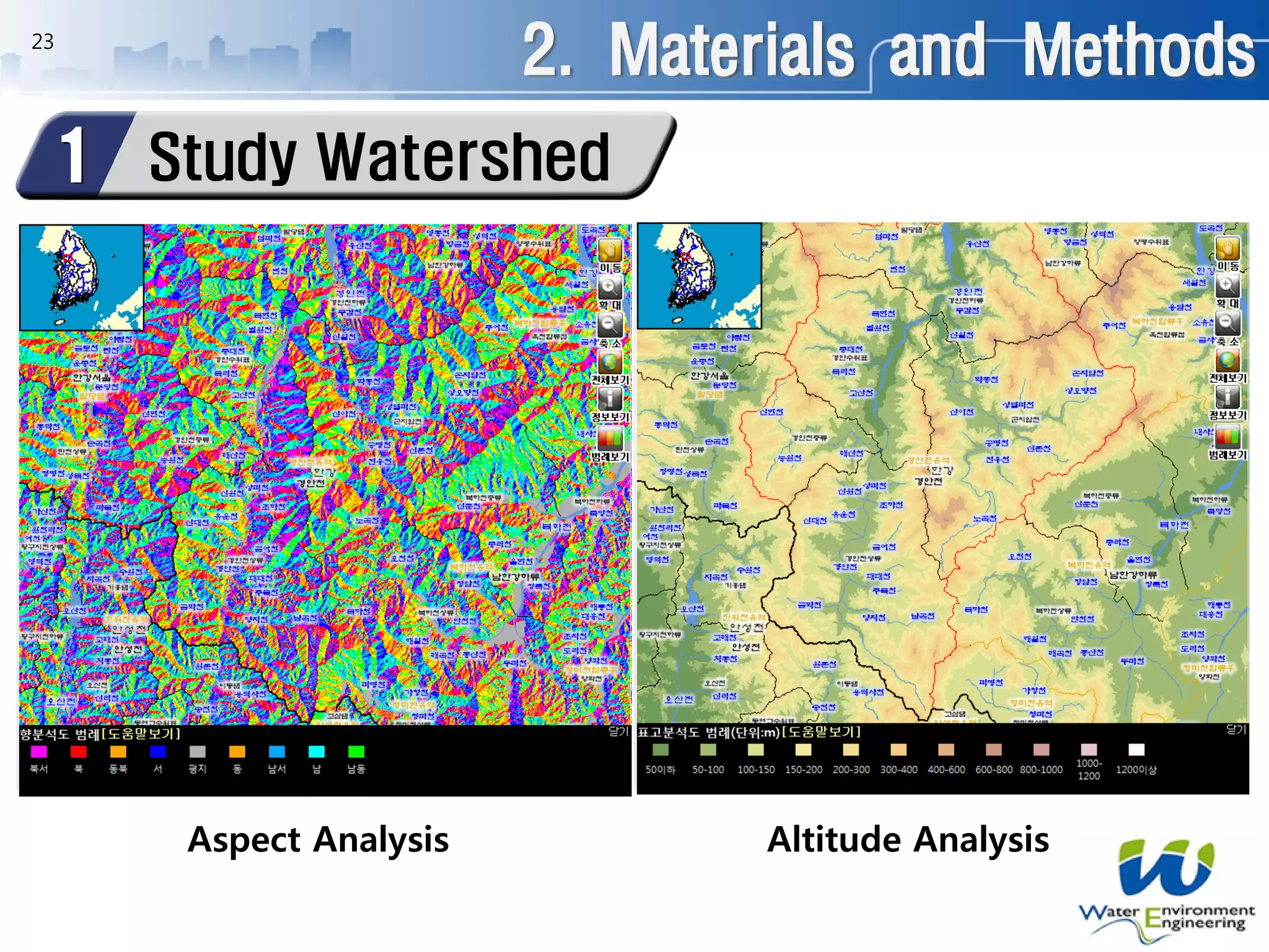
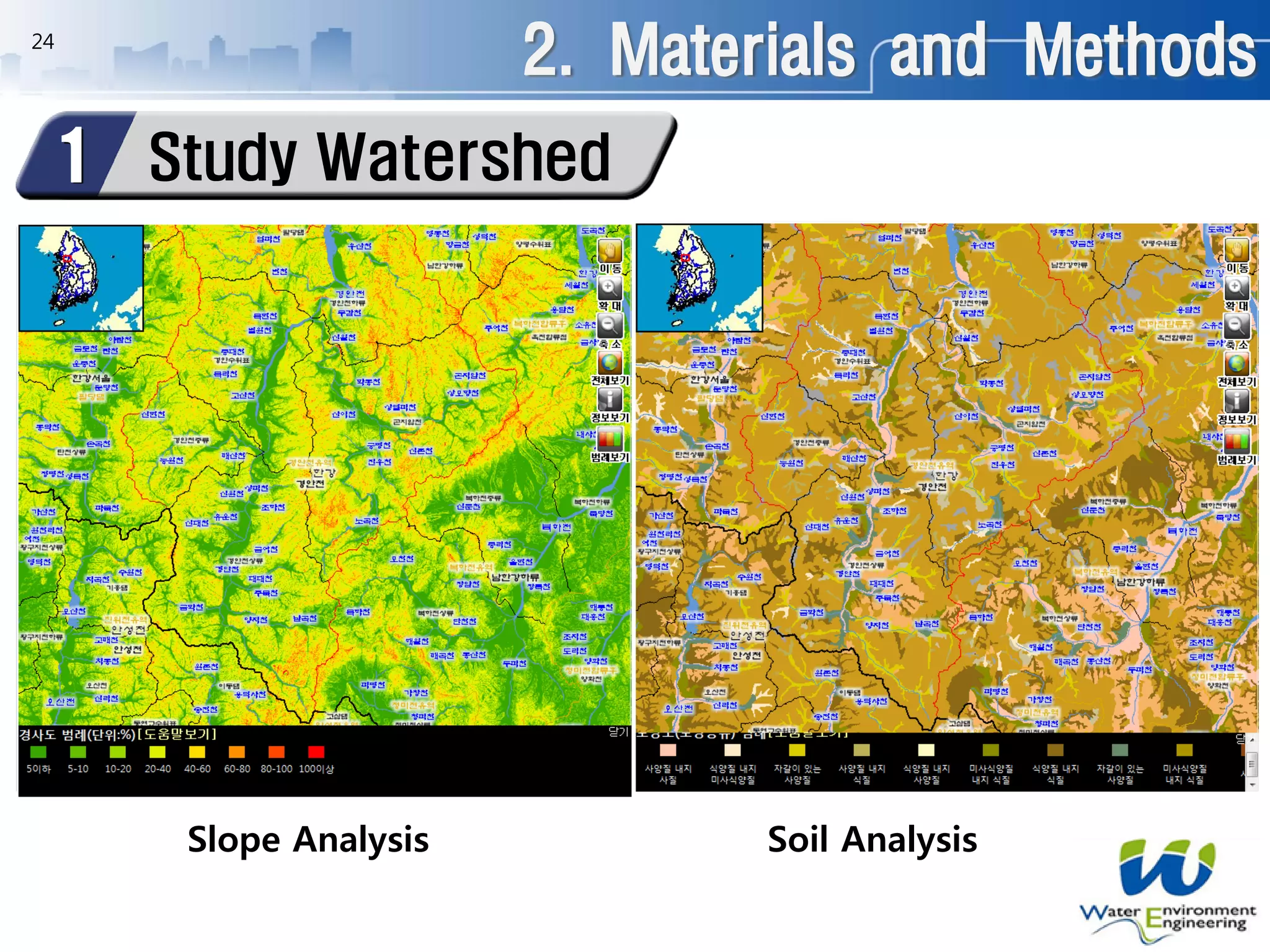
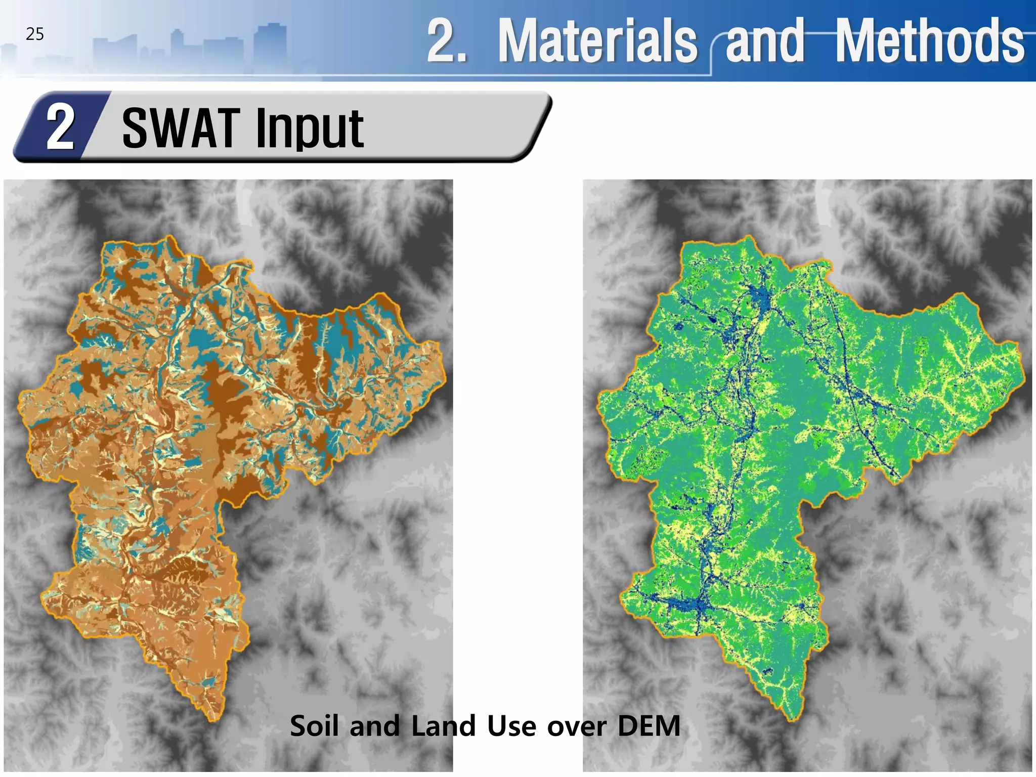
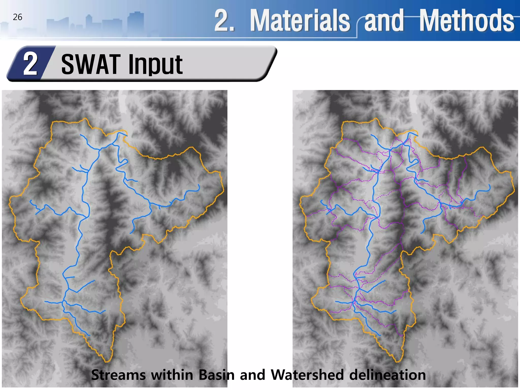
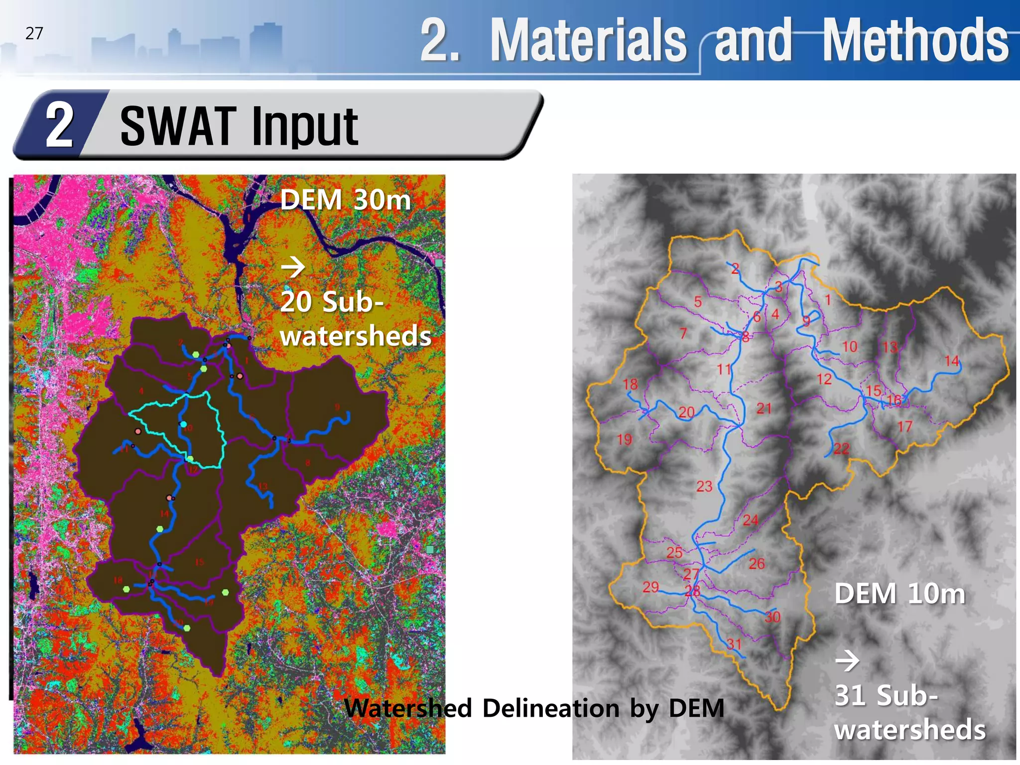
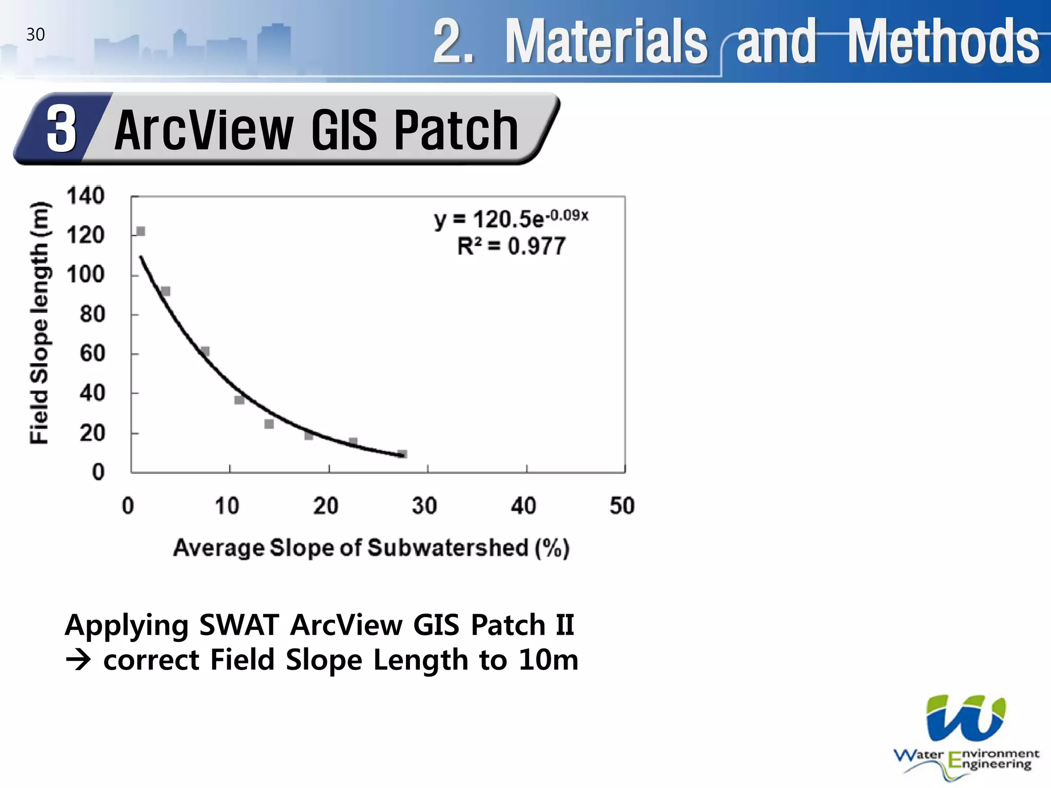
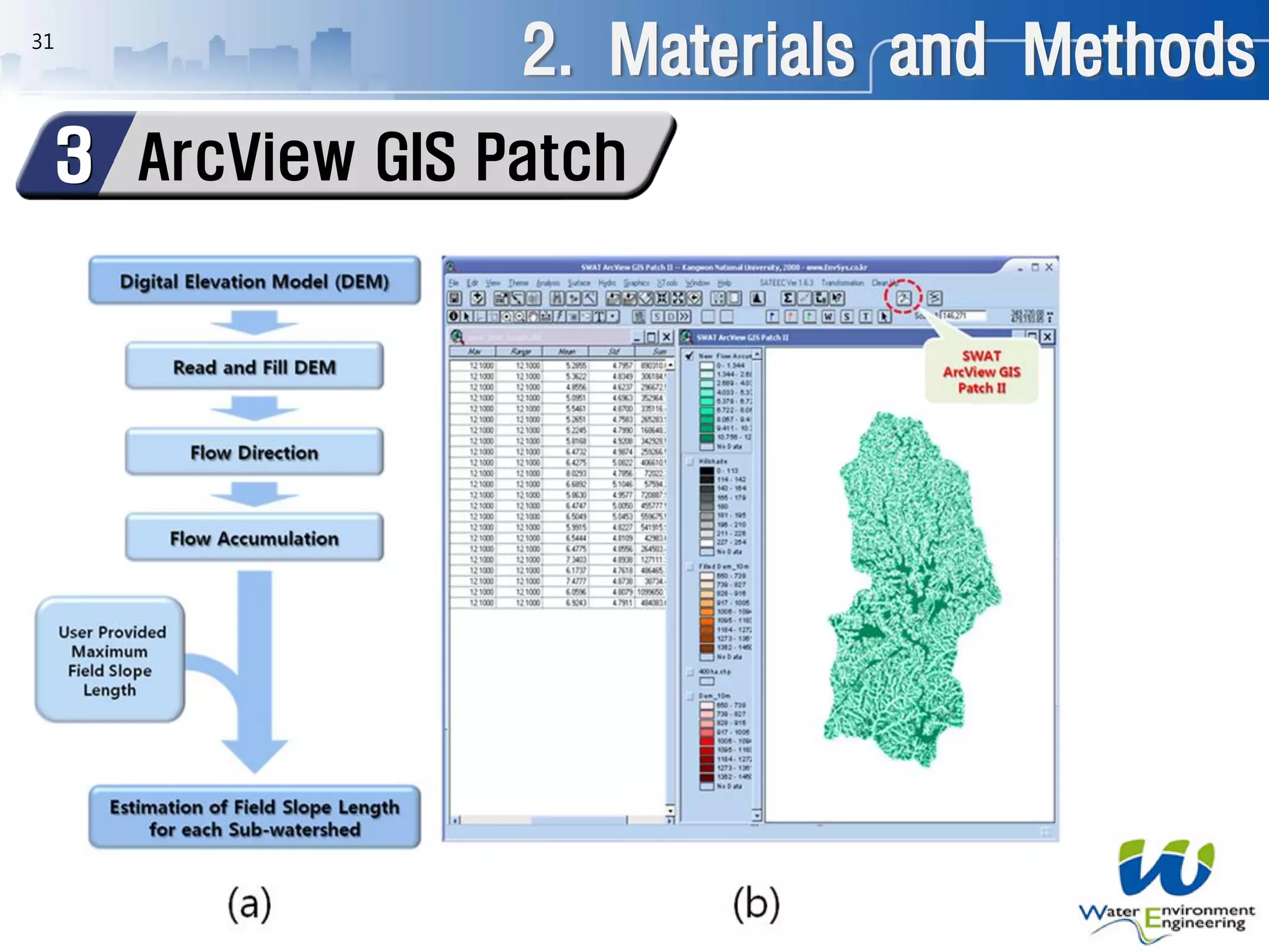
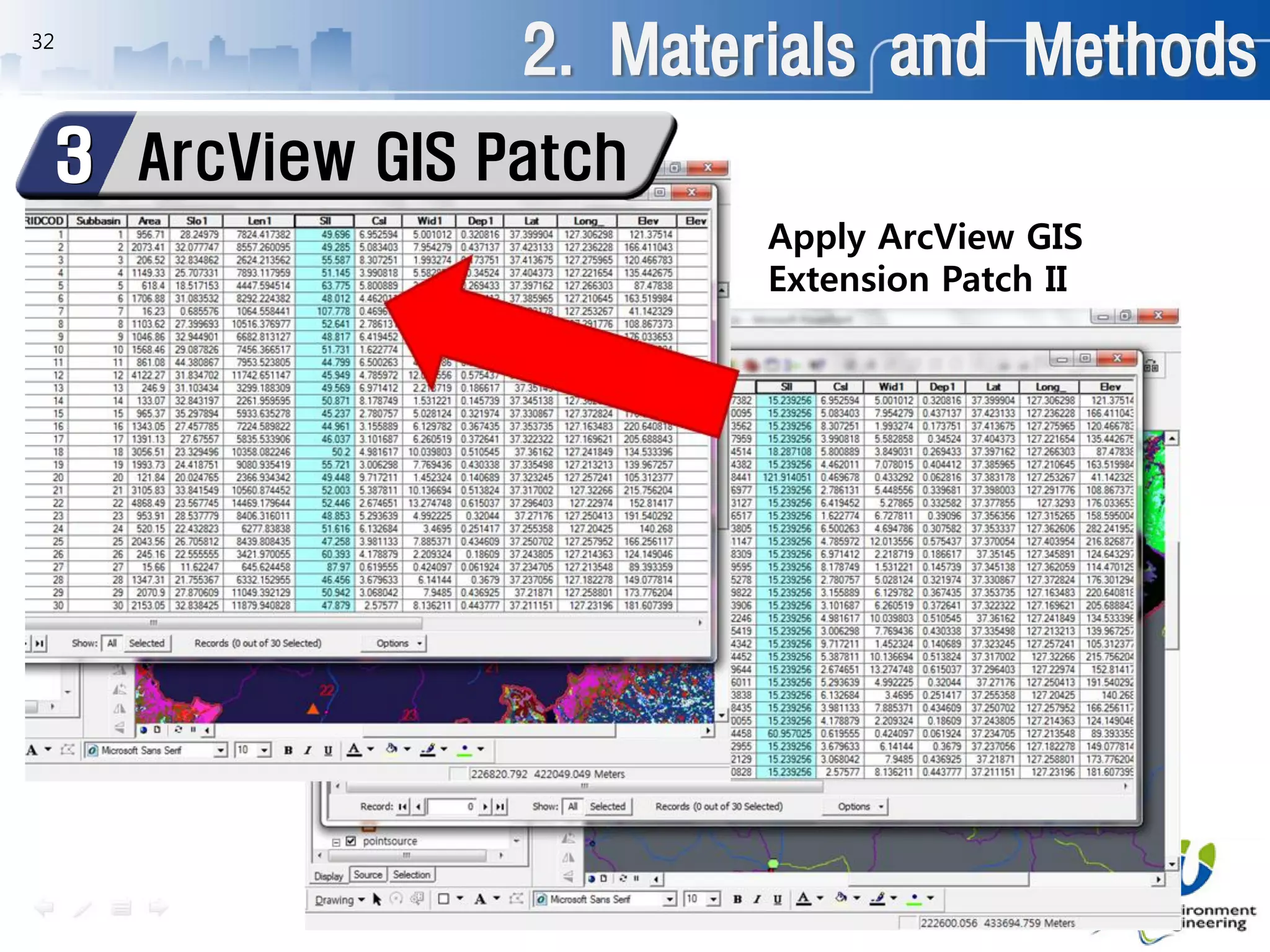
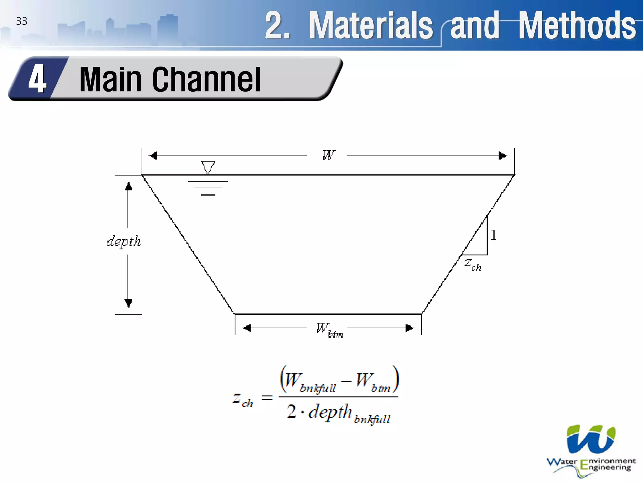
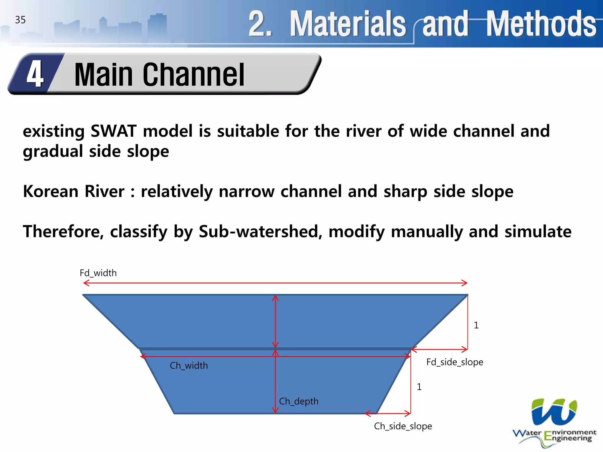
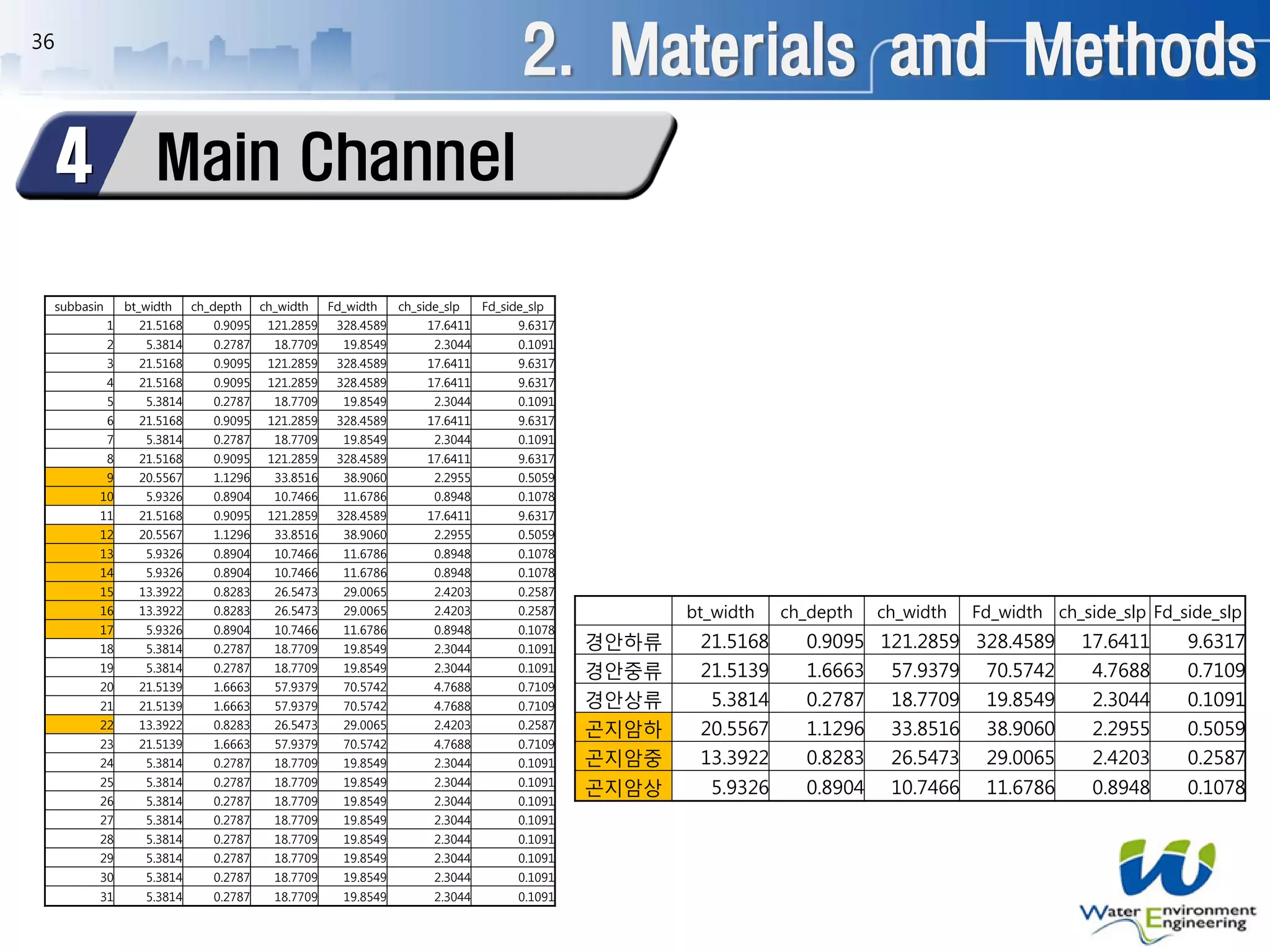
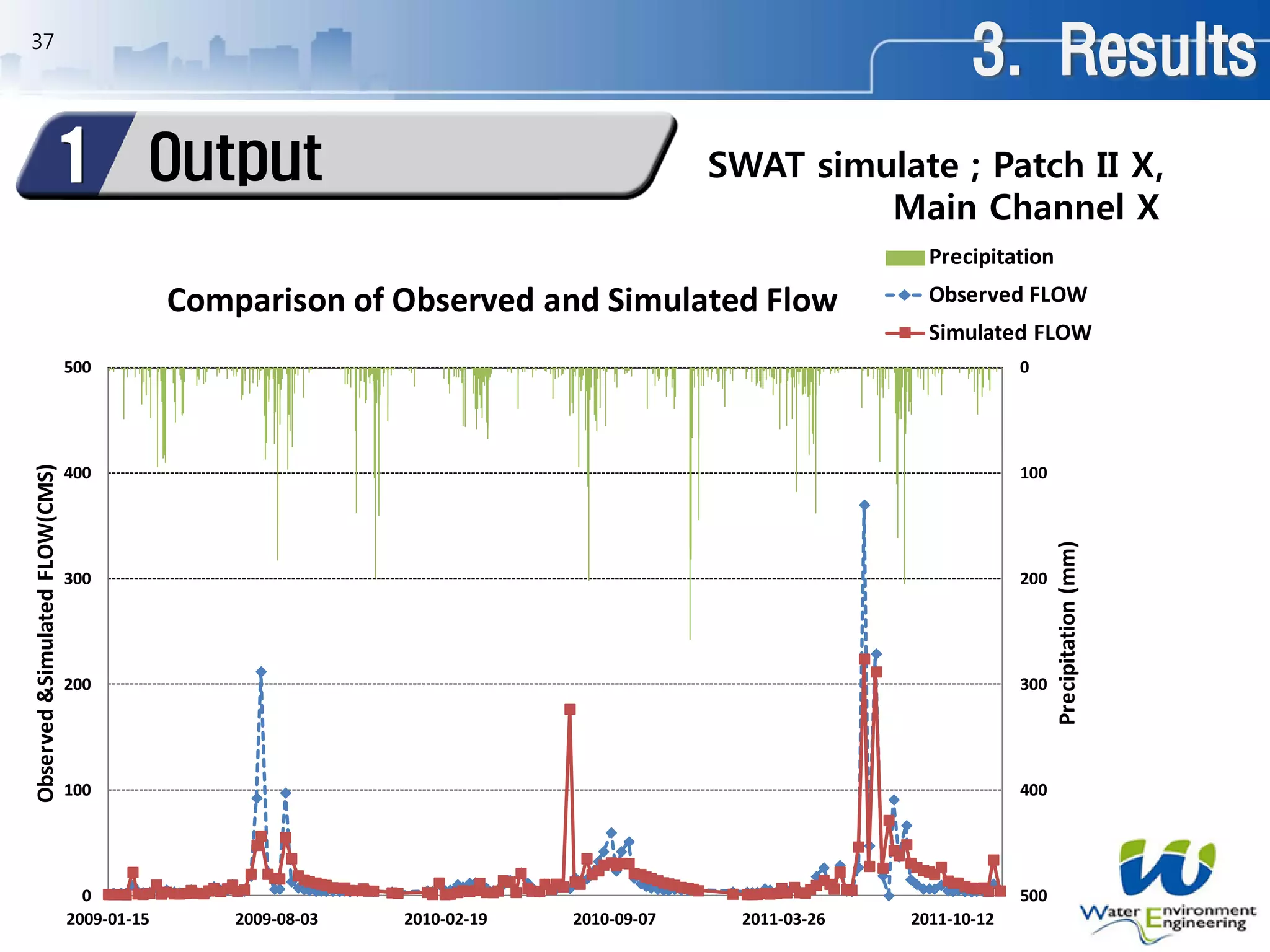
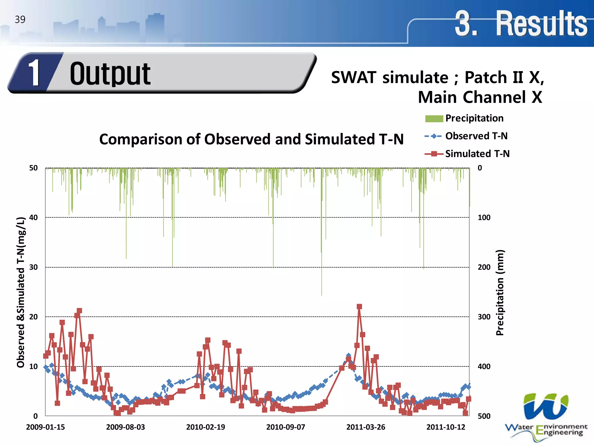
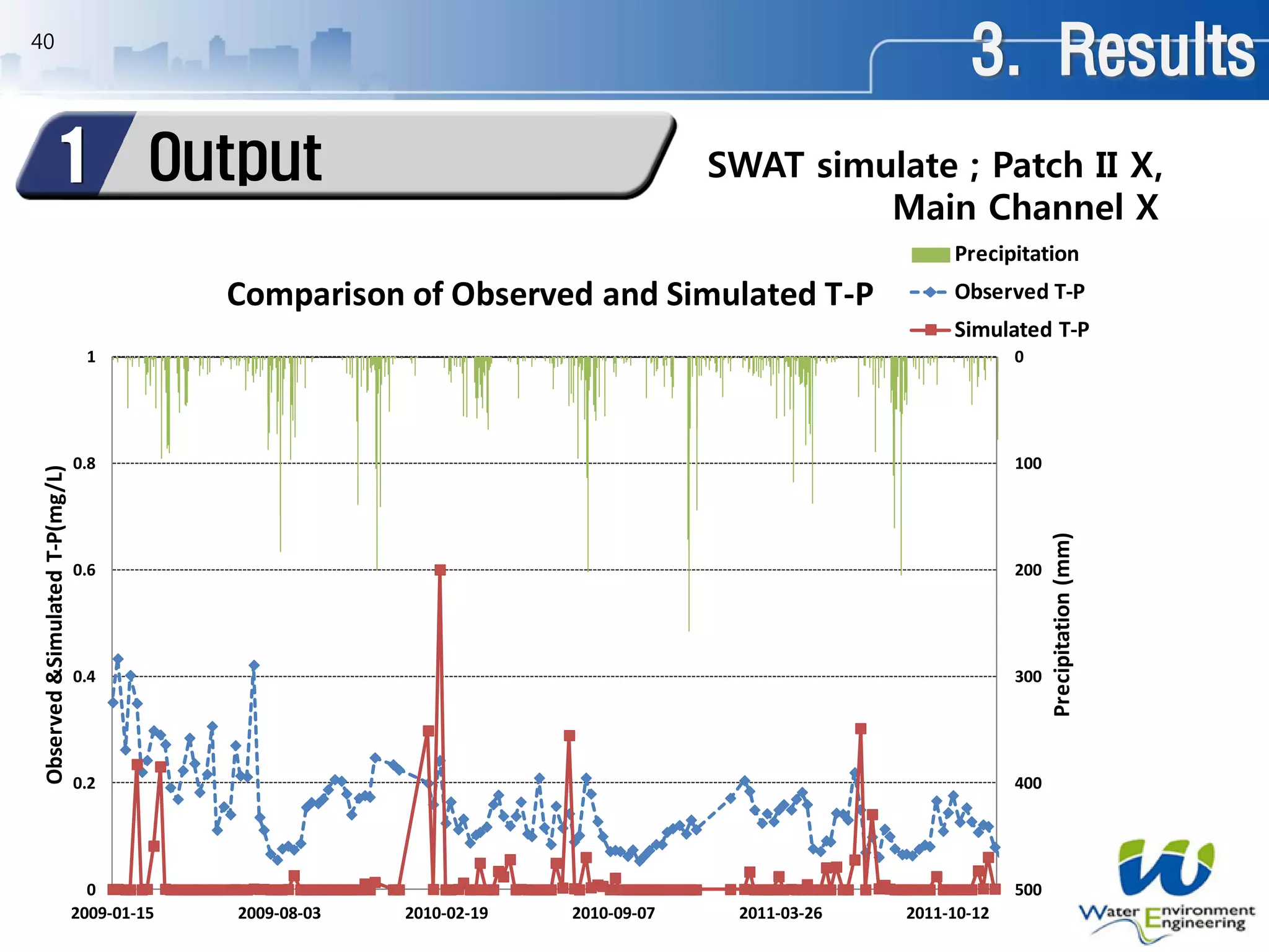
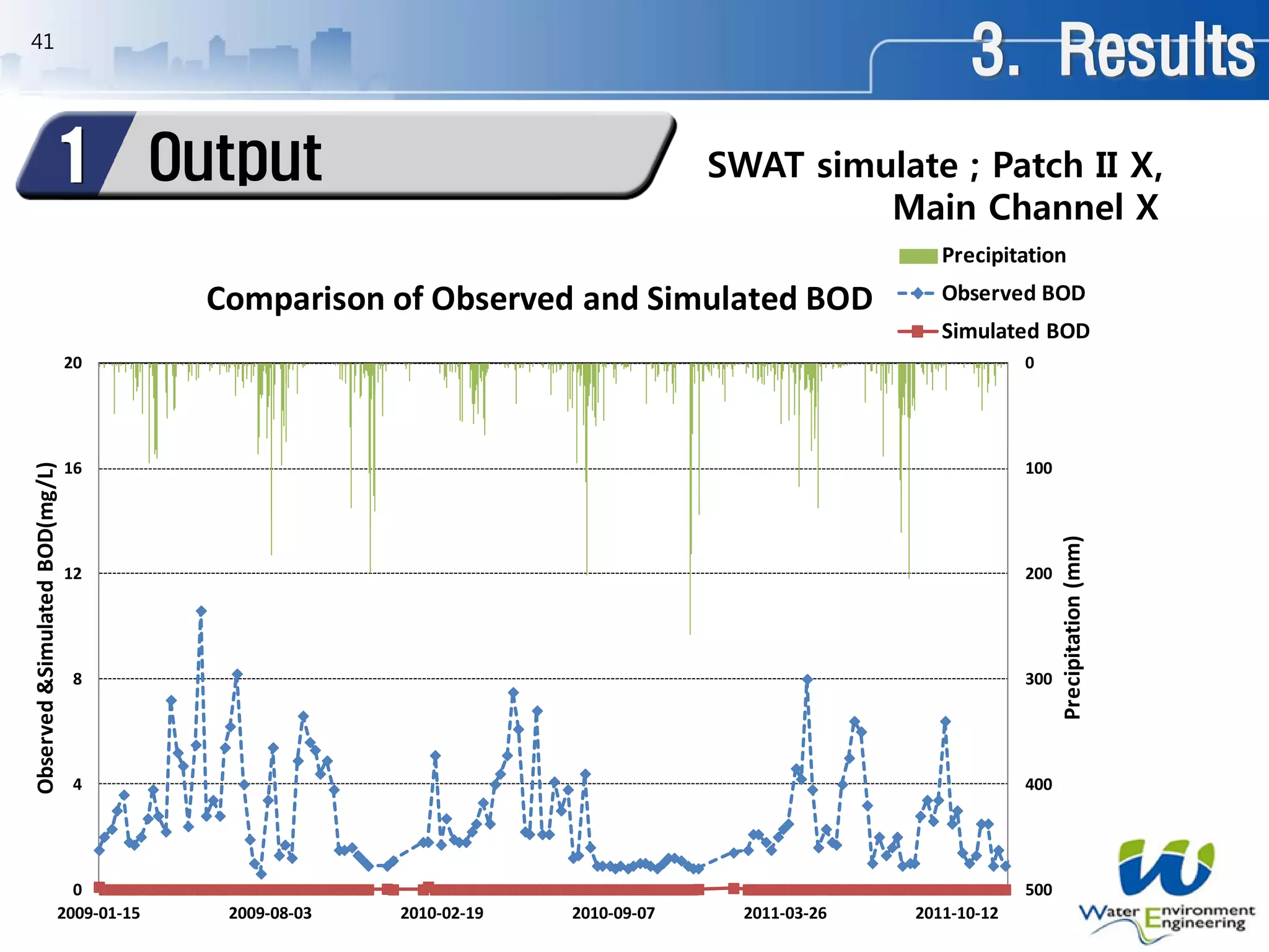
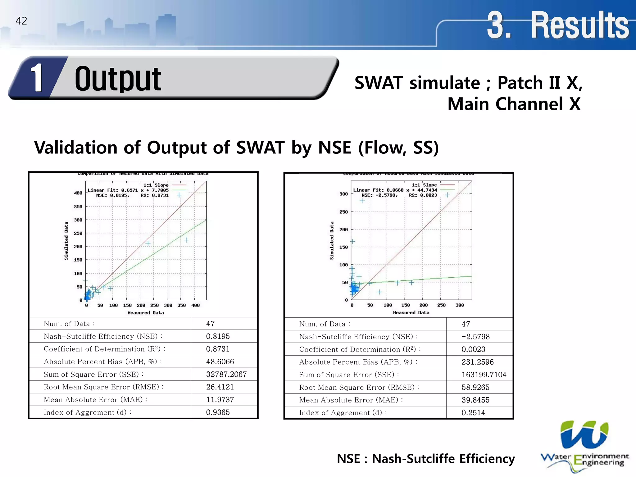
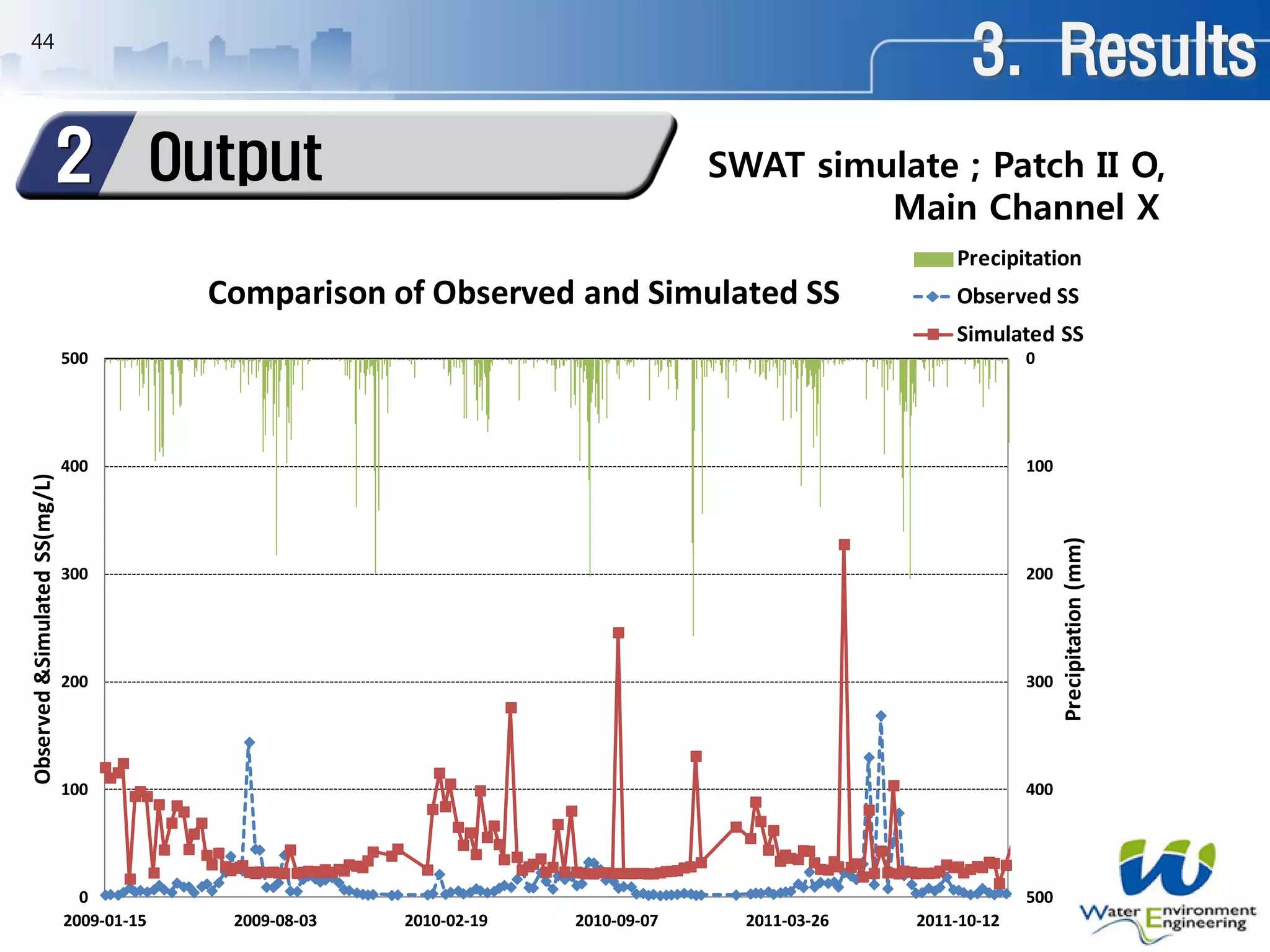
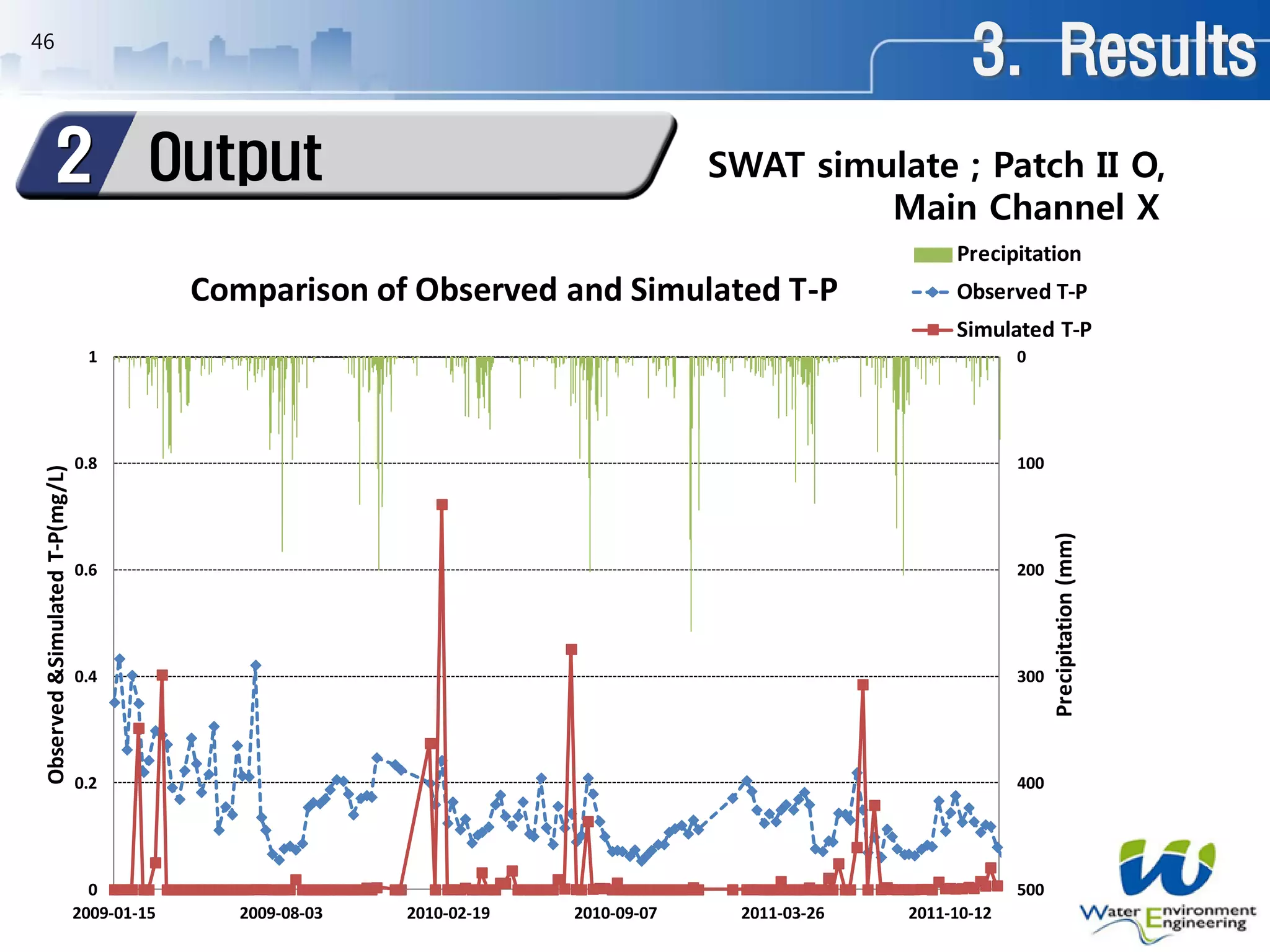
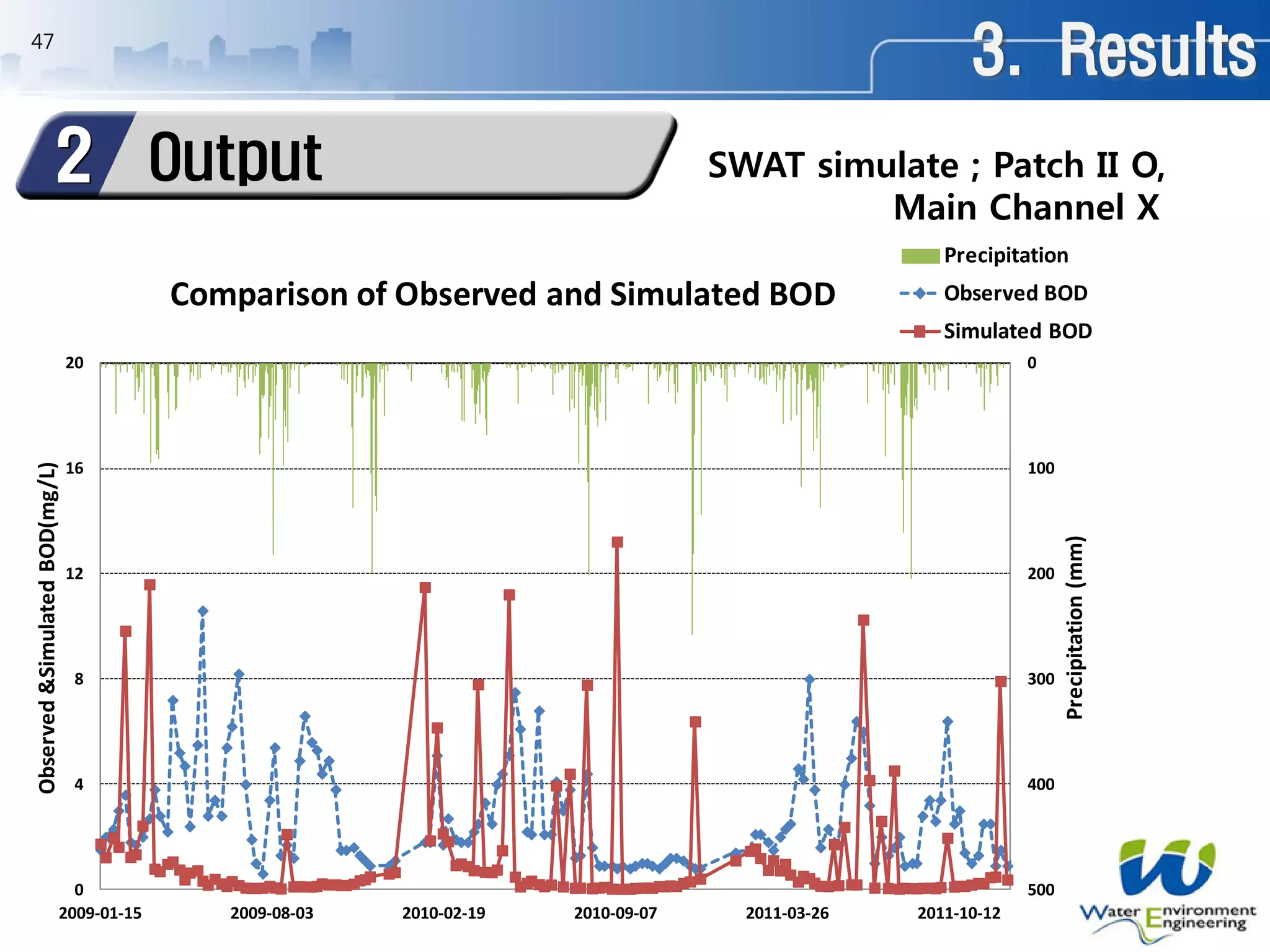
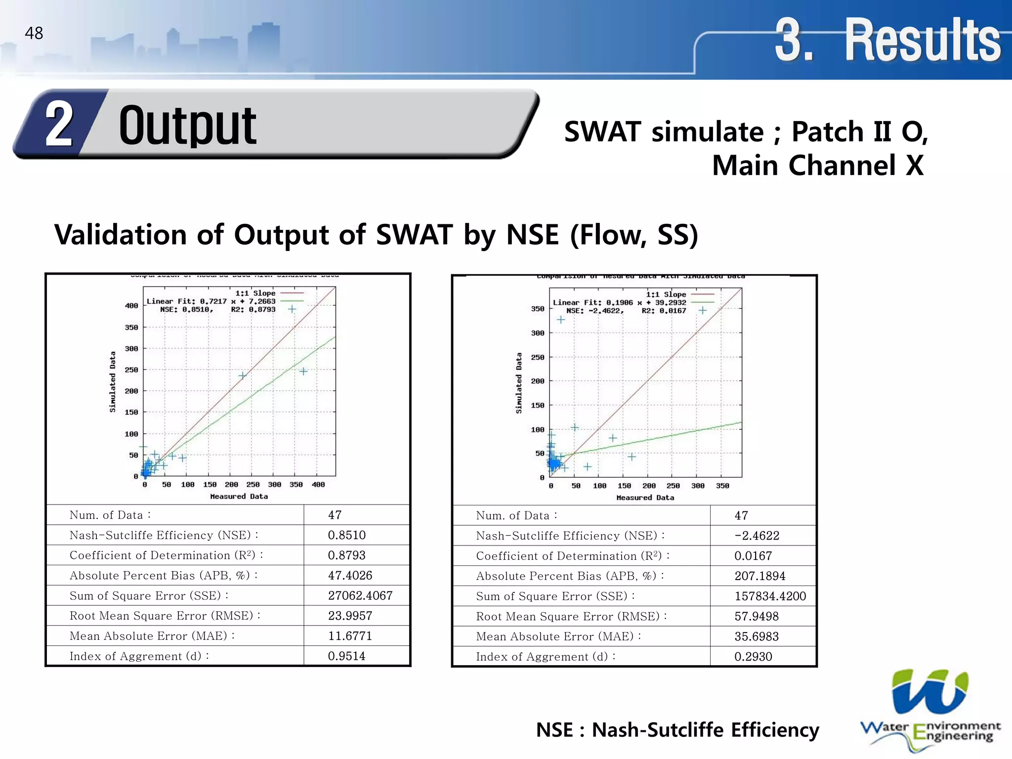
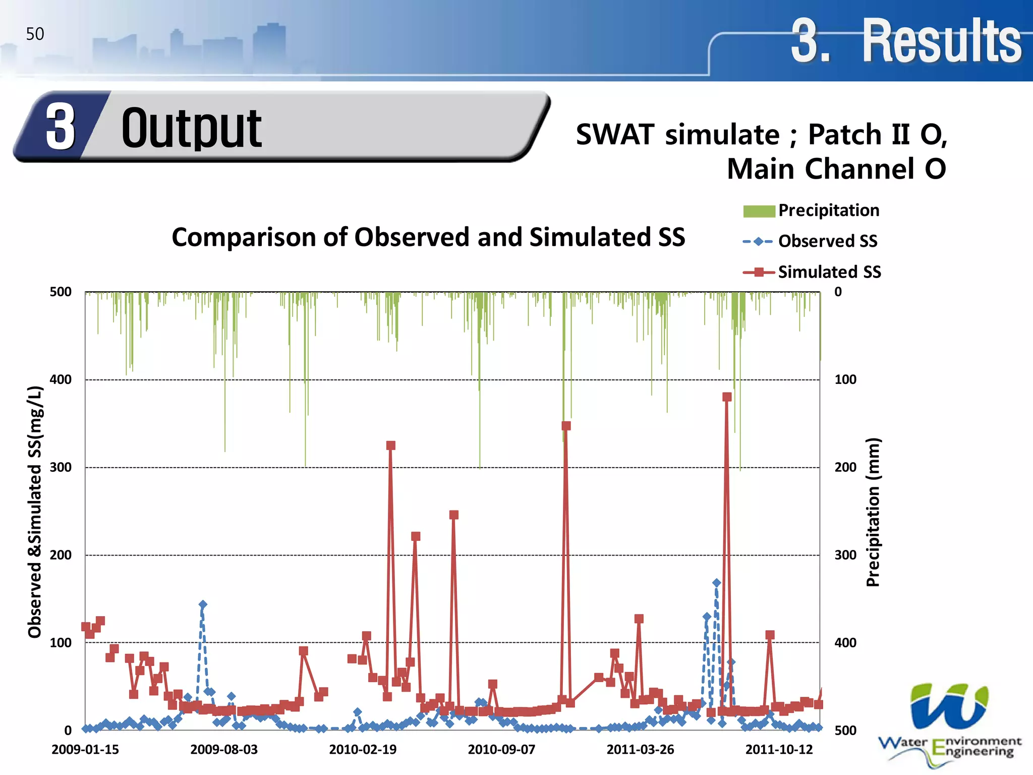
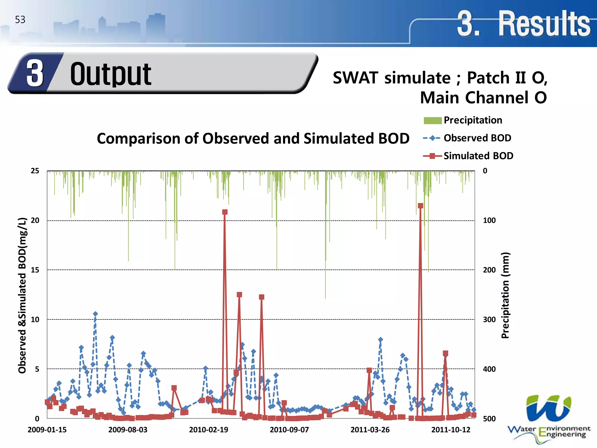
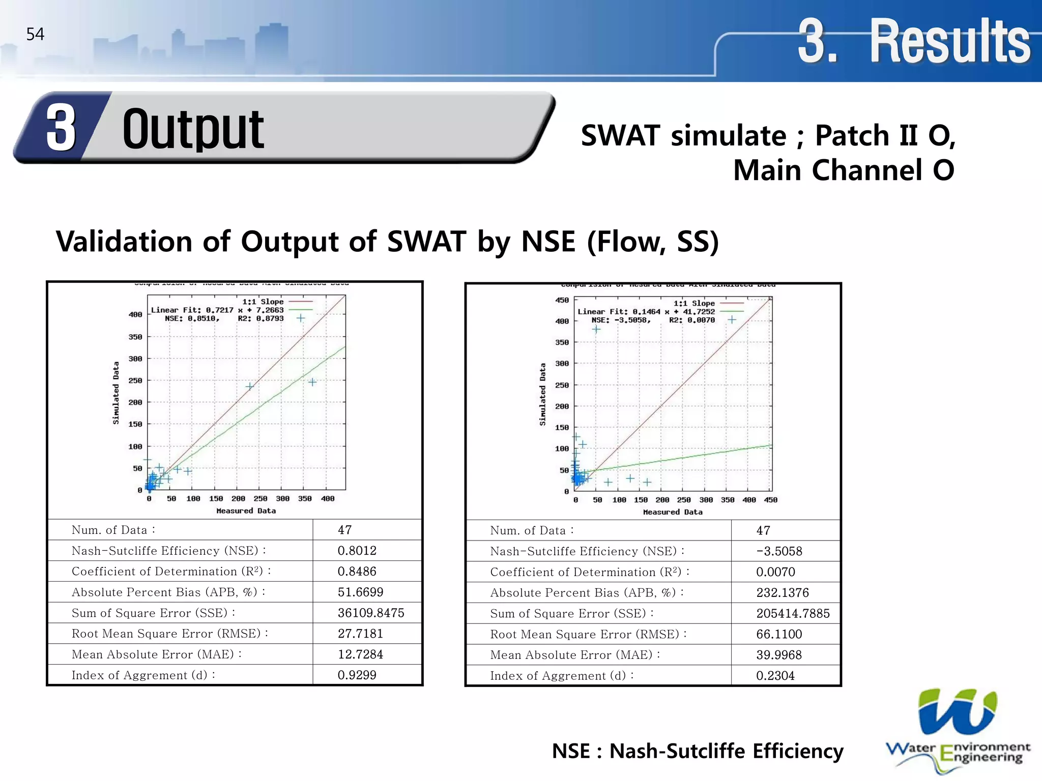
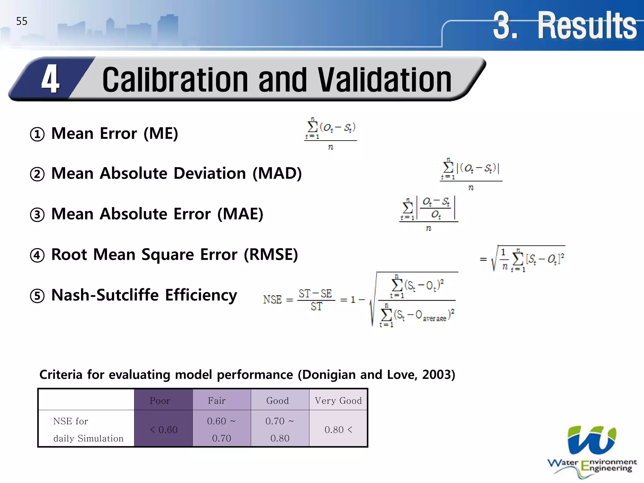
오염총량관리에 따른
GIS와 수질모델링에 의한
경안천 유역의
오염부하량 배출특성 연구
Study on Discharge Characteristics of Pollutant Load
at Gyoungahn River with GIS and Water Quality Modelling
for Total Maximum Loads Management
서울시립대학교
물 환 경 연 구 실 Lee, Kwan-Woo
E X
1. Introduction
2. Materials and Methods
3. Results
DI N
1. Introduction
Background1
Industrialization, Urbanization
 increase pollution loading on water supply source
As Management of Point Pollution Source enhanced
 Contribution rate of Non-point Pollution Source increased
Impose of Total Maximum Loads Management (‘99)
Ratio of Non-point Pollution Source in Discharge : about 42% (‘05)
3
1. Introduction
Background1
4
Discharge Loading By Pollution Source
1. Introduction
Background1
5
strengthen Effluent Standard, more Installation of Sewerage
 Point Source Loading decreased
Ratio of Discharge Loading by Non-point Pollution Source
increased
current Pollution Management reaches the limit
related Laws revised ;
Government demands Prediction and Countermeasure to
Developer
1. Introduction
Purpose1
6
Estimating Pollutant Load based on Land Use Plan, Precipitation
and Pollution Rate
 Hard to predict on Runoff Loading of actual Sub-watersheds
by Non-point Pollution Source
Non-point Pollution Source run off at rainfall
 Runoff flow vary on each Season,
therefore hard to predict, quantify
for more efficient Total Maximum Loads Management
require exact Pollution State
and Geographic Information System using Digital Elevation Model,
to analyze corresponding Water Basins
7
Purpose1
Input DATA
- GIS
DEM, Soils, Land Use
- Climate
Precipitation etc.
- Point Source
Sewage Treatment Plant
Wastewater Treatment Plant
SWAT Model
Output for each stream
- Flow
- Constituent Yields
Additional DATA
- Hydraulic, Hydrologic Coeff.
of Sub-watershed
- Slope Length
1. Introduction
1. Introduction
Purpose1
8
Research on Land Use Plan, Soil, Climate, Precipitation
 Input SWAT Model =
estimating Pollution Loads by Non-point Pollution Source
Research on Characteristic Data about Streams / River
 Input SWAT Model =
Slope Length Patch, Hydraulic / Hydrologic Coefficient
Analyzing Discharge Characteristics of Pollutant Load
 Apply to Policy, considering Priority
1. Introduction
Water Quality Modelling2
9
Using Water Quality Modelling for Total Maximum Loads
Management
- to decrease Conflict between local Governments
- to seek balanced Development between local Governments
Therefore,
Modelling required reasonable, fair, scientific Process
1. Introduction10
1) Procedure
- Setting up Purpose
- Understanding current State
- Setting up Scope
- Making Scenario
- Analyzing Prediction Results
2) Problem and Limit
- lack of fundamental Data or unsuitable
- not enough considering local Characteristics
- Uncertainty of Prediction
Water Quality Modelling2
1. Introduction
SWAT3
11
SWAT(Soil and Water Assessment Tool) is
River basin, or Watershed Scale Model
developed by USDA Agricultural Research Service)
to predict the impact of land management practices on water,
sediment and agricultural chemical yields
SWAT’s benefits are
Watersheds with no monitoring data can be modeled,
The relative impact of alternative input data on water quality
or other variables of interest can be quantified
SWAT is continuous time Model
1. Introduction
SWAT3
12
SWAT Input :
- Climate
Solar Radiation, Temperature, Wind Speed
Precipitation, Relative Humidity
- Hydrology
Surface Runoff, Evapotranspiration, Sub-surface Water, Groundwater
- Nutrients / Pesticides
Nitrogen, Phosphorus, Pesticides, Sediment, Nutrients, DO, CBOD
- Land Cover / Plant
- Main Channel Processes
Channel Characteristics, Flow rate and velocity
Preparation
1. Introduction
SWAT3
13
Schematic of SWAT Model
Input
- GIS
DEM, Soils, Land Use
- Climate
Temp., Relative Humidity, Precipitation etc.
- Point Source
Sewage Treatment Plant
Wastewater Treatment Plant
Effluent Water Quality Data
SWAT Model Analyze Output
Calibration
& Validation
1. Introduction
SWAT3
14
Schematic representation of the hydrologic cycle
Water Balance Equation
1. Introduction
SWAT3
15
1. Introduction
SWAT3
16
In-Stream Processes modeled by SWAT
1. Introduction
SWAT3
17
Partitioning of Nitrogen in SWAT
1. Introduction
SWAT3
18
Partitioning of Nitrogen in SWAT
1. Introduction
SWAT3
19
Partitioning of Phosphorous in SWAT
1. Introduction
SWAT3
20
Partitioning of Phosphorous in SWAT
2. Materials and Methods
Study Watershed1
21
Location of Gyoungahn River
Watershed Overview
2. Materials and Methods
Study Watershed1
22
Basin Length (km) Area (㎢) Sub-Watershed Area (㎢)
Gyoungahn
River
22.50 / 49.30 575.32
Gyoungahn A 198.4
Gyoungahn B 248.9
Location of Monitoring Site
2. Materials and Methods
Study Watershed1
23
Aspect Analysis Altitude Analysis
2. Materials and Methods
Study Watershed1
24
Slope Analysis Soil Analysis
25
2. Materials and Methods
SWAT Input2
Soil and Land Use over DEM
26
Streams within Basin and Watershed delineation
2. Materials and Methods
SWAT Input2
27
DEM 30m

20 Sub-
watersheds
DEM 10m

31 Sub-
watersheds
2. Materials and Methods
SWAT Input2
Watershed Delineation by DEM
2. Materials and Methods28
Streams within Basin Land Use and etc.
SWAT Input2
29
ArcView GIS Patch3
SWAT model calculates Average Slope using DEM,
simulates with Average Field Slope Length
existing SWAT model is developed that
use Field Slope Length as 0.05m
in the topography of average slope ≥ 25%
existing SWAT model is suitable for U.S. topography, in generally
gradual Slope
these condition is hard to apply to Korean topography, sharp
Slope
2. Materials and Methods
30
Applying SWAT ArcView GIS Patch II
 correct Field Slope Length to 10m
ArcView GIS Patch3
2. Materials and Methods
31
ArcView GIS Patch3
2. Materials and Methods
32
ArcView GIS Patch3
2. Materials and Methods
Apply ArcView GIS
Extension Patch II
33
Main Channel4
2. Materials and Methods
34
Main Channel4
2. Materials and Methods
35
Main Channel4
Ch_side_slope
Fd_side_slope
existing SWAT model is suitable for the river of wide channel and
gradual side slope
Korean River : relatively narrow channel and sharp side slope
Therefore, classify by Sub-watershed, modify manually and simulate
2. Materials and Methods
Fd_width
Ch_width
Ch_depth
1
1
36
2. Materials and Methods
Main Channel4
subbasin bt_width ch_depth ch_width Fd_width ch_side_slp Fd_side_slp
1 21.5168 0.9095 121.2859 328.4589 17.6411 9.6317
2 5.3814 0.2787 18.7709 19.8549 2.3044 0.1091
3 21.5168 0.9095 121.2859 328.4589 17.6411 9.6317
4 21.5168 0.9095 121.2859 328.4589 17.6411 9.6317
5 5.3814 0.2787 18.7709 19.8549 2.3044 0.1091
6 21.5168 0.9095 121.2859 328.4589 17.6411 9.6317
7 5.3814 0.2787 18.7709 19.8549 2.3044 0.1091
8 21.5168 0.9095 121.2859 328.4589 17.6411 9.6317
9 20.5567 1.1296 33.8516 38.9060 2.2955 0.5059
10 5.9326 0.8904 10.7466 11.6786 0.8948 0.1078
11 21.5168 0.9095 121.2859 328.4589 17.6411 9.6317
12 20.5567 1.1296 33.8516 38.9060 2.2955 0.5059
13 5.9326 0.8904 10.7466 11.6786 0.8948 0.1078
14 5.9326 0.8904 10.7466 11.6786 0.8948 0.1078
15 13.3922 0.8283 26.5473 29.0065 2.4203 0.2587
16 13.3922 0.8283 26.5473 29.0065 2.4203 0.2587
17 5.9326 0.8904 10.7466 11.6786 0.8948 0.1078
18 5.3814 0.2787 18.7709 19.8549 2.3044 0.1091
19 5.3814 0.2787 18.7709 19.8549 2.3044 0.1091
20 21.5139 1.6663 57.9379 70.5742 4.7688 0.7109
21 21.5139 1.6663 57.9379 70.5742 4.7688 0.7109
22 13.3922 0.8283 26.5473 29.0065 2.4203 0.2587
23 21.5139 1.6663 57.9379 70.5742 4.7688 0.7109
24 5.3814 0.2787 18.7709 19.8549 2.3044 0.1091
25 5.3814 0.2787 18.7709 19.8549 2.3044 0.1091
26 5.3814 0.2787 18.7709 19.8549 2.3044 0.1091
27 5.3814 0.2787 18.7709 19.8549 2.3044 0.1091
28 5.3814 0.2787 18.7709 19.8549 2.3044 0.1091
29 5.3814 0.2787 18.7709 19.8549 2.3044 0.1091
30 5.3814 0.2787 18.7709 19.8549 2.3044 0.1091
31 5.3814 0.2787 18.7709 19.8549 2.3044 0.1091
bt_width ch_depth ch_width Fd_width ch_side_slp Fd_side_slp
경안하류 21.5168 0.9095 121.2859 328.4589 17.6411 9.6317
경안중류 21.5139 1.6663 57.9379 70.5742 4.7688 0.7109
경안상류 5.3814 0.2787 18.7709 19.8549 2.3044 0.1091
곤지암하 20.5567 1.1296 33.8516 38.9060 2.2955 0.5059
곤지암중 13.3922 0.8283 26.5473 29.0065 2.4203 0.2587
곤지암상 5.9326 0.8904 10.7466 11.6786 0.8948 0.1078
37
3. Results
Output1
0
100
200
300
400
5000
100
200
300
400
500
2009-01-15 2009-08-03 2010-02-19 2010-09-07 2011-03-26 2011-10-12
Precipitation(mm)
Observed&SimulatedFLOW(CMS)
Comparison of Observed and Simulated Flow
Precipitation
Observed FLOW
Simulated FLOW
SWAT simulate ; Patch II X,
Main Channel X
38
0
100
200
300
400
5000
100
200
300
400
500
2009-01-15 2009-08-03 2010-02-19 2010-09-07 2011-03-26 2011-10-12
Precipitation(mm)
Observed&SimulatedSS(mg/L)
Comparison of Observed and Simulated SS
Precipitation
Observed SS
Simulated SS
SWAT simulate ; Patch II X,
Main Channel X
3. Results
Output1
39
0
100
200
300
400
5000
10
20
30
40
50
2009-01-15 2009-08-03 2010-02-19 2010-09-07 2011-03-26 2011-10-12
Precipitation(mm)
Observed&SimulatedT-N(mg/L)
Comparison of Observed and Simulated T-N
Precipitation
Observed T-N
Simulated T-N
SWAT simulate ; Patch II X,
Main Channel X
3. Results
Output1
40
0
100
200
300
400
5000
0.2
0.4
0.6
0.8
1
2009-01-15 2009-08-03 2010-02-19 2010-09-07 2011-03-26 2011-10-12
Precipitation(mm)
Observed&SimulatedT-P(mg/L)
Comparison of Observed and Simulated T-P
Precipitation
Observed T-P
Simulated T-P
SWAT simulate ; Patch II X,
Main Channel X
3. Results
Output1
41
0
100
200
300
400
5000
4
8
12
16
20
2009-01-15 2009-08-03 2010-02-19 2010-09-07 2011-03-26 2011-10-12
Precipitation(mm)
Observed&SimulatedBOD(mg/L)
Comparison of Observed and Simulated BOD
Precipitation
Observed BOD
Simulated BOD
SWAT simulate ; Patch II X,
Main Channel X
3. Results
Output1
42
Num. of Data : 47
Nash-Sutcliffe Efficiency (NSE) : 0.8195
Coefficient of Determination (R2) : 0.8731
Absolute Percent Bias (APB, %) : 48.6066
Sum of Square Error (SSE) : 32787.2067
Root Mean Square Error (RMSE) : 26.4121
Mean Absolute Error (MAE) : 11.9737
Index of Aggrement (d) : 0.9365
Num. of Data : 47
Nash-Sutcliffe Efficiency (NSE) : -2.5798
Coefficient of Determination (R2) : 0.0023
Absolute Percent Bias (APB, %) : 231.2596
Sum of Square Error (SSE) : 163199.7104
Root Mean Square Error (RMSE) : 58.9265
Mean Absolute Error (MAE) : 39.8455
Index of Aggrement (d) : 0.2514
Validation of Output of SWAT by NSE (Flow, SS)
SWAT simulate ; Patch II X,
Main Channel X
3. Results
Output1
NSE : Nash-Sutcliffe Efficiency
43
0
100
200
300
400
5000
100
200
300
400
500
2009-01-15 2009-08-03 2010-02-19 2010-09-07 2011-03-26 2011-10-12
Precipitation(mm)
Observed&SimulatedFLOW(CMS)
Comparison of Observed and Simulated Flow
Precipitation
Observed FLOW
Simulated FLOW
SWAT simulate ; Patch II O,
Main Channel X
3. Results
Output2
44
0
100
200
300
400
5000
100
200
300
400
500
2009-01-15 2009-08-03 2010-02-19 2010-09-07 2011-03-26 2011-10-12
Precipitation(mm)
Observed&SimulatedSS(mg/L)
Comparison of Observed and Simulated SS
Precipitation
Observed SS
Simulated SS
SWAT simulate ; Patch II O,
Main Channel X
3. Results
Output2
45
0
100
200
300
400
5000
10
20
30
40
50
2009-01-15 2009-08-03 2010-02-19 2010-09-07 2011-03-26 2011-10-12
Precipitation(mm)
Observed&SimulatedT-N(mg/L)
Comparison of Observed and Simulated T-N
Precipitation
Observed T-N
Simulated T-N
SWAT simulate ; Patch II O,
Main Channel X
3. Results
Output2
46
0
100
200
300
400
5000
0.2
0.4
0.6
0.8
1
2009-01-15 2009-08-03 2010-02-19 2010-09-07 2011-03-26 2011-10-12
Precipitation(mm)
Observed&SimulatedT-P(mg/L)
Comparison of Observed and Simulated T-P
Precipitation
Observed T-P
Simulated T-P
SWAT simulate ; Patch II O,
Main Channel X
3. Results
Output2
47
0
100
200
300
400
5000
4
8
12
16
20
2009-01-15 2009-08-03 2010-02-19 2010-09-07 2011-03-26 2011-10-12
Precipitation(mm)
Observed&SimulatedBOD(mg/L)
Comparison of Observed and Simulated BOD
Precipitation
Observed BOD
Simulated BOD
SWAT simulate ; Patch II O,
Main Channel X
3. Results
Output2
48
Num. of Data : 47
Nash-Sutcliffe Efficiency (NSE) : 0.8510
Coefficient of Determination (R2) : 0.8793
Absolute Percent Bias (APB, %) : 47.4026
Sum of Square Error (SSE) : 27062.4067
Root Mean Square Error (RMSE) : 23.9957
Mean Absolute Error (MAE) : 11.6771
Index of Aggrement (d) : 0.9514
Num. of Data : 47
Nash-Sutcliffe Efficiency (NSE) : -2.4622
Coefficient of Determination (R2) : 0.0167
Absolute Percent Bias (APB, %) : 207.1894
Sum of Square Error (SSE) : 157834.4200
Root Mean Square Error (RMSE) : 57.9498
Mean Absolute Error (MAE) : 35.6983
Index of Aggrement (d) : 0.2930
SWAT simulate ; Patch II O,
Main Channel X
3. Results
Output2
Validation of Output of SWAT by NSE (Flow, SS)
NSE : Nash-Sutcliffe Efficiency
49
0
100
200
300
400
5000
100
200
300
400
500
2009-01-15 2009-08-03 2010-02-19 2010-09-07 2011-03-26 2011-10-12
Precipitation(mm)
Observed&SimulatedFLOW(CMS)
Comparison of Observed and Simulated Flow
Precipitation
Observed FLOW
Simulated FLOW
SWAT simulate ; Patch II O,
Main Channel O
3. Results
Output3
50
0
100
200
300
400
5000
100
200
300
400
500
2009-01-15 2009-08-03 2010-02-19 2010-09-07 2011-03-26 2011-10-12
Precipitation(mm)
Observed&SimulatedSS(mg/L)
Comparison of Observed and Simulated SS
Precipitation
Observed SS
Simulated SS
SWAT simulate ; Patch II O,
Main Channel O
3. Results
Output3
51
0
100
200
300
400
5000
10
20
30
40
50
2009-01-15 2009-08-03 2010-02-19 2010-09-07 2011-03-26 2011-10-12
Precipitation(mm)
Observed&SimulatedT-N(mg/L)
Comparison of Observed and Simulated T-N
Precipitation
Observed T-N
Simulated T-N
SWAT simulate ; Patch II O,
Main Channel O
3. Results
Output3
52
0
100
200
300
400
5000
0.2
0.4
0.6
0.8
1
2009-01-15 2009-08-03 2010-02-19 2010-09-07 2011-03-26 2011-10-12
Precipitation(mm)
Observed&SimulatedT-P(mg/L)
Comparison of Observed and Simulated T-P
Precipitation
Observed T-P
Simulated T-P
SWAT simulate ; Patch II O,
Main Channel O
3. Results
Output3
53
0
100
200
300
400
5000
5
10
15
20
25
2009-01-15 2009-08-03 2010-02-19 2010-09-07 2011-03-26 2011-10-12
Precipitation(mm)
Observed&SimulatedBOD(mg/L)
Comparison of Observed and Simulated BOD
Precipitation
Observed BOD
Simulated BOD
SWAT simulate ; Patch II O,
Main Channel O
3. Results
Output3
54
Num. of Data : 47
Nash-Sutcliffe Efficiency (NSE) : 0.8012
Coefficient of Determination (R2) : 0.8486
Absolute Percent Bias (APB, %) : 51.6699
Sum of Square Error (SSE) : 36109.8475
Root Mean Square Error (RMSE) : 27.7181
Mean Absolute Error (MAE) : 12.7284
Index of Aggrement (d) : 0.9299
Num. of Data : 47
Nash-Sutcliffe Efficiency (NSE) : -3.5058
Coefficient of Determination (R2) : 0.0070
Absolute Percent Bias (APB, %) : 232.1376
Sum of Square Error (SSE) : 205414.7885
Root Mean Square Error (RMSE) : 66.1100
Mean Absolute Error (MAE) : 39.9968
Index of Aggrement (d) : 0.2304
SWAT simulate ; Patch II O,
Main Channel O
Output3
Validation of Output of SWAT by NSE (Flow, SS)
NSE : Nash-Sutcliffe Efficiency
3. Results
55
Calibration and Validation4
① Mean Error (ME)
② Mean Absolute Deviation (MAD)
③ Mean Absolute Error (MAE)
④ Root Mean Square Error (RMSE)
⑤ Nash-Sutcliffe Efficiency
Poor Fair Good Very Good
NSE for
daily Simulation
< 0.60
0.60 ~
0.70
0.70 ~
0.80
0.80 <
Criteria for evaluating model performance (Donigian and Love, 2003)
3. Results
56
Calibration and Validation4
3. Results

Study on Discharge Characteristics of Pollutant Load at Gyoungahn River with GIS and Water Quality Modelling for Total Maximum Loads Management

  • 1.
    오염총량관리에 따른 GIS와 수질모델링에의한 경안천 유역의 오염부하량 배출특성 연구 Study on Discharge Characteristics of Pollutant Load at Gyoungahn River with GIS and Water Quality Modelling for Total Maximum Loads Management 서울시립대학교 물 환 경 연 구 실 Lee, Kwan-Woo
  • 2.
    E X 1. Introduction 2.Materials and Methods 3. Results DI N
  • 3.
    1. Introduction Background1 Industrialization, Urbanization increase pollution loading on water supply source As Management of Point Pollution Source enhanced  Contribution rate of Non-point Pollution Source increased Impose of Total Maximum Loads Management (‘99) Ratio of Non-point Pollution Source in Discharge : about 42% (‘05) 3
  • 4.
  • 5.
    1. Introduction Background1 5 strengthen EffluentStandard, more Installation of Sewerage  Point Source Loading decreased Ratio of Discharge Loading by Non-point Pollution Source increased current Pollution Management reaches the limit related Laws revised ; Government demands Prediction and Countermeasure to Developer
  • 6.
    1. Introduction Purpose1 6 Estimating PollutantLoad based on Land Use Plan, Precipitation and Pollution Rate  Hard to predict on Runoff Loading of actual Sub-watersheds by Non-point Pollution Source Non-point Pollution Source run off at rainfall  Runoff flow vary on each Season, therefore hard to predict, quantify for more efficient Total Maximum Loads Management require exact Pollution State and Geographic Information System using Digital Elevation Model, to analyze corresponding Water Basins
  • 7.
    7 Purpose1 Input DATA - GIS DEM,Soils, Land Use - Climate Precipitation etc. - Point Source Sewage Treatment Plant Wastewater Treatment Plant SWAT Model Output for each stream - Flow - Constituent Yields Additional DATA - Hydraulic, Hydrologic Coeff. of Sub-watershed - Slope Length 1. Introduction
  • 8.
    1. Introduction Purpose1 8 Research onLand Use Plan, Soil, Climate, Precipitation  Input SWAT Model = estimating Pollution Loads by Non-point Pollution Source Research on Characteristic Data about Streams / River  Input SWAT Model = Slope Length Patch, Hydraulic / Hydrologic Coefficient Analyzing Discharge Characteristics of Pollutant Load  Apply to Policy, considering Priority
  • 9.
    1. Introduction Water QualityModelling2 9 Using Water Quality Modelling for Total Maximum Loads Management - to decrease Conflict between local Governments - to seek balanced Development between local Governments Therefore, Modelling required reasonable, fair, scientific Process
  • 10.
    1. Introduction10 1) Procedure -Setting up Purpose - Understanding current State - Setting up Scope - Making Scenario - Analyzing Prediction Results 2) Problem and Limit - lack of fundamental Data or unsuitable - not enough considering local Characteristics - Uncertainty of Prediction Water Quality Modelling2
  • 11.
    1. Introduction SWAT3 11 SWAT(Soil andWater Assessment Tool) is River basin, or Watershed Scale Model developed by USDA Agricultural Research Service) to predict the impact of land management practices on water, sediment and agricultural chemical yields SWAT’s benefits are Watersheds with no monitoring data can be modeled, The relative impact of alternative input data on water quality or other variables of interest can be quantified SWAT is continuous time Model
  • 12.
    1. Introduction SWAT3 12 SWAT Input: - Climate Solar Radiation, Temperature, Wind Speed Precipitation, Relative Humidity - Hydrology Surface Runoff, Evapotranspiration, Sub-surface Water, Groundwater - Nutrients / Pesticides Nitrogen, Phosphorus, Pesticides, Sediment, Nutrients, DO, CBOD - Land Cover / Plant - Main Channel Processes Channel Characteristics, Flow rate and velocity
  • 13.
    Preparation 1. Introduction SWAT3 13 Schematic ofSWAT Model Input - GIS DEM, Soils, Land Use - Climate Temp., Relative Humidity, Precipitation etc. - Point Source Sewage Treatment Plant Wastewater Treatment Plant Effluent Water Quality Data SWAT Model Analyze Output Calibration & Validation
  • 14.
  • 15.
    Water Balance Equation 1.Introduction SWAT3 15
  • 16.
  • 17.
  • 18.
  • 19.
  • 20.
  • 21.
    2. Materials andMethods Study Watershed1 21 Location of Gyoungahn River
  • 22.
    Watershed Overview 2. Materialsand Methods Study Watershed1 22 Basin Length (km) Area (㎢) Sub-Watershed Area (㎢) Gyoungahn River 22.50 / 49.30 575.32 Gyoungahn A 198.4 Gyoungahn B 248.9 Location of Monitoring Site
  • 23.
    2. Materials andMethods Study Watershed1 23 Aspect Analysis Altitude Analysis
  • 24.
    2. Materials andMethods Study Watershed1 24 Slope Analysis Soil Analysis
  • 25.
    25 2. Materials andMethods SWAT Input2 Soil and Land Use over DEM
  • 26.
    26 Streams within Basinand Watershed delineation 2. Materials and Methods SWAT Input2
  • 27.
    27 DEM 30m  20 Sub- watersheds DEM10m  31 Sub- watersheds 2. Materials and Methods SWAT Input2 Watershed Delineation by DEM
  • 28.
    2. Materials andMethods28 Streams within Basin Land Use and etc. SWAT Input2
  • 29.
    29 ArcView GIS Patch3 SWATmodel calculates Average Slope using DEM, simulates with Average Field Slope Length existing SWAT model is developed that use Field Slope Length as 0.05m in the topography of average slope ≥ 25% existing SWAT model is suitable for U.S. topography, in generally gradual Slope these condition is hard to apply to Korean topography, sharp Slope 2. Materials and Methods
  • 30.
    30 Applying SWAT ArcViewGIS Patch II  correct Field Slope Length to 10m ArcView GIS Patch3 2. Materials and Methods
  • 31.
    31 ArcView GIS Patch3 2.Materials and Methods
  • 32.
    32 ArcView GIS Patch3 2.Materials and Methods Apply ArcView GIS Extension Patch II
  • 33.
  • 34.
  • 35.
    35 Main Channel4 Ch_side_slope Fd_side_slope existing SWATmodel is suitable for the river of wide channel and gradual side slope Korean River : relatively narrow channel and sharp side slope Therefore, classify by Sub-watershed, modify manually and simulate 2. Materials and Methods Fd_width Ch_width Ch_depth 1 1
  • 36.
    36 2. Materials andMethods Main Channel4 subbasin bt_width ch_depth ch_width Fd_width ch_side_slp Fd_side_slp 1 21.5168 0.9095 121.2859 328.4589 17.6411 9.6317 2 5.3814 0.2787 18.7709 19.8549 2.3044 0.1091 3 21.5168 0.9095 121.2859 328.4589 17.6411 9.6317 4 21.5168 0.9095 121.2859 328.4589 17.6411 9.6317 5 5.3814 0.2787 18.7709 19.8549 2.3044 0.1091 6 21.5168 0.9095 121.2859 328.4589 17.6411 9.6317 7 5.3814 0.2787 18.7709 19.8549 2.3044 0.1091 8 21.5168 0.9095 121.2859 328.4589 17.6411 9.6317 9 20.5567 1.1296 33.8516 38.9060 2.2955 0.5059 10 5.9326 0.8904 10.7466 11.6786 0.8948 0.1078 11 21.5168 0.9095 121.2859 328.4589 17.6411 9.6317 12 20.5567 1.1296 33.8516 38.9060 2.2955 0.5059 13 5.9326 0.8904 10.7466 11.6786 0.8948 0.1078 14 5.9326 0.8904 10.7466 11.6786 0.8948 0.1078 15 13.3922 0.8283 26.5473 29.0065 2.4203 0.2587 16 13.3922 0.8283 26.5473 29.0065 2.4203 0.2587 17 5.9326 0.8904 10.7466 11.6786 0.8948 0.1078 18 5.3814 0.2787 18.7709 19.8549 2.3044 0.1091 19 5.3814 0.2787 18.7709 19.8549 2.3044 0.1091 20 21.5139 1.6663 57.9379 70.5742 4.7688 0.7109 21 21.5139 1.6663 57.9379 70.5742 4.7688 0.7109 22 13.3922 0.8283 26.5473 29.0065 2.4203 0.2587 23 21.5139 1.6663 57.9379 70.5742 4.7688 0.7109 24 5.3814 0.2787 18.7709 19.8549 2.3044 0.1091 25 5.3814 0.2787 18.7709 19.8549 2.3044 0.1091 26 5.3814 0.2787 18.7709 19.8549 2.3044 0.1091 27 5.3814 0.2787 18.7709 19.8549 2.3044 0.1091 28 5.3814 0.2787 18.7709 19.8549 2.3044 0.1091 29 5.3814 0.2787 18.7709 19.8549 2.3044 0.1091 30 5.3814 0.2787 18.7709 19.8549 2.3044 0.1091 31 5.3814 0.2787 18.7709 19.8549 2.3044 0.1091 bt_width ch_depth ch_width Fd_width ch_side_slp Fd_side_slp 경안하류 21.5168 0.9095 121.2859 328.4589 17.6411 9.6317 경안중류 21.5139 1.6663 57.9379 70.5742 4.7688 0.7109 경안상류 5.3814 0.2787 18.7709 19.8549 2.3044 0.1091 곤지암하 20.5567 1.1296 33.8516 38.9060 2.2955 0.5059 곤지암중 13.3922 0.8283 26.5473 29.0065 2.4203 0.2587 곤지암상 5.9326 0.8904 10.7466 11.6786 0.8948 0.1078
  • 37.
    37 3. Results Output1 0 100 200 300 400 5000 100 200 300 400 500 2009-01-15 2009-08-032010-02-19 2010-09-07 2011-03-26 2011-10-12 Precipitation(mm) Observed&SimulatedFLOW(CMS) Comparison of Observed and Simulated Flow Precipitation Observed FLOW Simulated FLOW SWAT simulate ; Patch II X, Main Channel X
  • 38.
    38 0 100 200 300 400 5000 100 200 300 400 500 2009-01-15 2009-08-03 2010-02-192010-09-07 2011-03-26 2011-10-12 Precipitation(mm) Observed&SimulatedSS(mg/L) Comparison of Observed and Simulated SS Precipitation Observed SS Simulated SS SWAT simulate ; Patch II X, Main Channel X 3. Results Output1
  • 39.
    39 0 100 200 300 400 5000 10 20 30 40 50 2009-01-15 2009-08-03 2010-02-192010-09-07 2011-03-26 2011-10-12 Precipitation(mm) Observed&SimulatedT-N(mg/L) Comparison of Observed and Simulated T-N Precipitation Observed T-N Simulated T-N SWAT simulate ; Patch II X, Main Channel X 3. Results Output1
  • 40.
    40 0 100 200 300 400 5000 0.2 0.4 0.6 0.8 1 2009-01-15 2009-08-03 2010-02-192010-09-07 2011-03-26 2011-10-12 Precipitation(mm) Observed&SimulatedT-P(mg/L) Comparison of Observed and Simulated T-P Precipitation Observed T-P Simulated T-P SWAT simulate ; Patch II X, Main Channel X 3. Results Output1
  • 41.
    41 0 100 200 300 400 5000 4 8 12 16 20 2009-01-15 2009-08-03 2010-02-192010-09-07 2011-03-26 2011-10-12 Precipitation(mm) Observed&SimulatedBOD(mg/L) Comparison of Observed and Simulated BOD Precipitation Observed BOD Simulated BOD SWAT simulate ; Patch II X, Main Channel X 3. Results Output1
  • 42.
    42 Num. of Data: 47 Nash-Sutcliffe Efficiency (NSE) : 0.8195 Coefficient of Determination (R2) : 0.8731 Absolute Percent Bias (APB, %) : 48.6066 Sum of Square Error (SSE) : 32787.2067 Root Mean Square Error (RMSE) : 26.4121 Mean Absolute Error (MAE) : 11.9737 Index of Aggrement (d) : 0.9365 Num. of Data : 47 Nash-Sutcliffe Efficiency (NSE) : -2.5798 Coefficient of Determination (R2) : 0.0023 Absolute Percent Bias (APB, %) : 231.2596 Sum of Square Error (SSE) : 163199.7104 Root Mean Square Error (RMSE) : 58.9265 Mean Absolute Error (MAE) : 39.8455 Index of Aggrement (d) : 0.2514 Validation of Output of SWAT by NSE (Flow, SS) SWAT simulate ; Patch II X, Main Channel X 3. Results Output1 NSE : Nash-Sutcliffe Efficiency
  • 43.
    43 0 100 200 300 400 5000 100 200 300 400 500 2009-01-15 2009-08-03 2010-02-192010-09-07 2011-03-26 2011-10-12 Precipitation(mm) Observed&SimulatedFLOW(CMS) Comparison of Observed and Simulated Flow Precipitation Observed FLOW Simulated FLOW SWAT simulate ; Patch II O, Main Channel X 3. Results Output2
  • 44.
    44 0 100 200 300 400 5000 100 200 300 400 500 2009-01-15 2009-08-03 2010-02-192010-09-07 2011-03-26 2011-10-12 Precipitation(mm) Observed&SimulatedSS(mg/L) Comparison of Observed and Simulated SS Precipitation Observed SS Simulated SS SWAT simulate ; Patch II O, Main Channel X 3. Results Output2
  • 45.
    45 0 100 200 300 400 5000 10 20 30 40 50 2009-01-15 2009-08-03 2010-02-192010-09-07 2011-03-26 2011-10-12 Precipitation(mm) Observed&SimulatedT-N(mg/L) Comparison of Observed and Simulated T-N Precipitation Observed T-N Simulated T-N SWAT simulate ; Patch II O, Main Channel X 3. Results Output2
  • 46.
    46 0 100 200 300 400 5000 0.2 0.4 0.6 0.8 1 2009-01-15 2009-08-03 2010-02-192010-09-07 2011-03-26 2011-10-12 Precipitation(mm) Observed&SimulatedT-P(mg/L) Comparison of Observed and Simulated T-P Precipitation Observed T-P Simulated T-P SWAT simulate ; Patch II O, Main Channel X 3. Results Output2
  • 47.
    47 0 100 200 300 400 5000 4 8 12 16 20 2009-01-15 2009-08-03 2010-02-192010-09-07 2011-03-26 2011-10-12 Precipitation(mm) Observed&SimulatedBOD(mg/L) Comparison of Observed and Simulated BOD Precipitation Observed BOD Simulated BOD SWAT simulate ; Patch II O, Main Channel X 3. Results Output2
  • 48.
    48 Num. of Data: 47 Nash-Sutcliffe Efficiency (NSE) : 0.8510 Coefficient of Determination (R2) : 0.8793 Absolute Percent Bias (APB, %) : 47.4026 Sum of Square Error (SSE) : 27062.4067 Root Mean Square Error (RMSE) : 23.9957 Mean Absolute Error (MAE) : 11.6771 Index of Aggrement (d) : 0.9514 Num. of Data : 47 Nash-Sutcliffe Efficiency (NSE) : -2.4622 Coefficient of Determination (R2) : 0.0167 Absolute Percent Bias (APB, %) : 207.1894 Sum of Square Error (SSE) : 157834.4200 Root Mean Square Error (RMSE) : 57.9498 Mean Absolute Error (MAE) : 35.6983 Index of Aggrement (d) : 0.2930 SWAT simulate ; Patch II O, Main Channel X 3. Results Output2 Validation of Output of SWAT by NSE (Flow, SS) NSE : Nash-Sutcliffe Efficiency
  • 49.
    49 0 100 200 300 400 5000 100 200 300 400 500 2009-01-15 2009-08-03 2010-02-192010-09-07 2011-03-26 2011-10-12 Precipitation(mm) Observed&SimulatedFLOW(CMS) Comparison of Observed and Simulated Flow Precipitation Observed FLOW Simulated FLOW SWAT simulate ; Patch II O, Main Channel O 3. Results Output3
  • 50.
    50 0 100 200 300 400 5000 100 200 300 400 500 2009-01-15 2009-08-03 2010-02-192010-09-07 2011-03-26 2011-10-12 Precipitation(mm) Observed&SimulatedSS(mg/L) Comparison of Observed and Simulated SS Precipitation Observed SS Simulated SS SWAT simulate ; Patch II O, Main Channel O 3. Results Output3
  • 51.
    51 0 100 200 300 400 5000 10 20 30 40 50 2009-01-15 2009-08-03 2010-02-192010-09-07 2011-03-26 2011-10-12 Precipitation(mm) Observed&SimulatedT-N(mg/L) Comparison of Observed and Simulated T-N Precipitation Observed T-N Simulated T-N SWAT simulate ; Patch II O, Main Channel O 3. Results Output3
  • 52.
    52 0 100 200 300 400 5000 0.2 0.4 0.6 0.8 1 2009-01-15 2009-08-03 2010-02-192010-09-07 2011-03-26 2011-10-12 Precipitation(mm) Observed&SimulatedT-P(mg/L) Comparison of Observed and Simulated T-P Precipitation Observed T-P Simulated T-P SWAT simulate ; Patch II O, Main Channel O 3. Results Output3
  • 53.
    53 0 100 200 300 400 5000 5 10 15 20 25 2009-01-15 2009-08-03 2010-02-192010-09-07 2011-03-26 2011-10-12 Precipitation(mm) Observed&SimulatedBOD(mg/L) Comparison of Observed and Simulated BOD Precipitation Observed BOD Simulated BOD SWAT simulate ; Patch II O, Main Channel O 3. Results Output3
  • 54.
    54 Num. of Data: 47 Nash-Sutcliffe Efficiency (NSE) : 0.8012 Coefficient of Determination (R2) : 0.8486 Absolute Percent Bias (APB, %) : 51.6699 Sum of Square Error (SSE) : 36109.8475 Root Mean Square Error (RMSE) : 27.7181 Mean Absolute Error (MAE) : 12.7284 Index of Aggrement (d) : 0.9299 Num. of Data : 47 Nash-Sutcliffe Efficiency (NSE) : -3.5058 Coefficient of Determination (R2) : 0.0070 Absolute Percent Bias (APB, %) : 232.1376 Sum of Square Error (SSE) : 205414.7885 Root Mean Square Error (RMSE) : 66.1100 Mean Absolute Error (MAE) : 39.9968 Index of Aggrement (d) : 0.2304 SWAT simulate ; Patch II O, Main Channel O Output3 Validation of Output of SWAT by NSE (Flow, SS) NSE : Nash-Sutcliffe Efficiency 3. Results
  • 55.
    55 Calibration and Validation4 ①Mean Error (ME) ② Mean Absolute Deviation (MAD) ③ Mean Absolute Error (MAE) ④ Root Mean Square Error (RMSE) ⑤ Nash-Sutcliffe Efficiency Poor Fair Good Very Good NSE for daily Simulation < 0.60 0.60 ~ 0.70 0.70 ~ 0.80 0.80 < Criteria for evaluating model performance (Donigian and Love, 2003) 3. Results
  • 56.