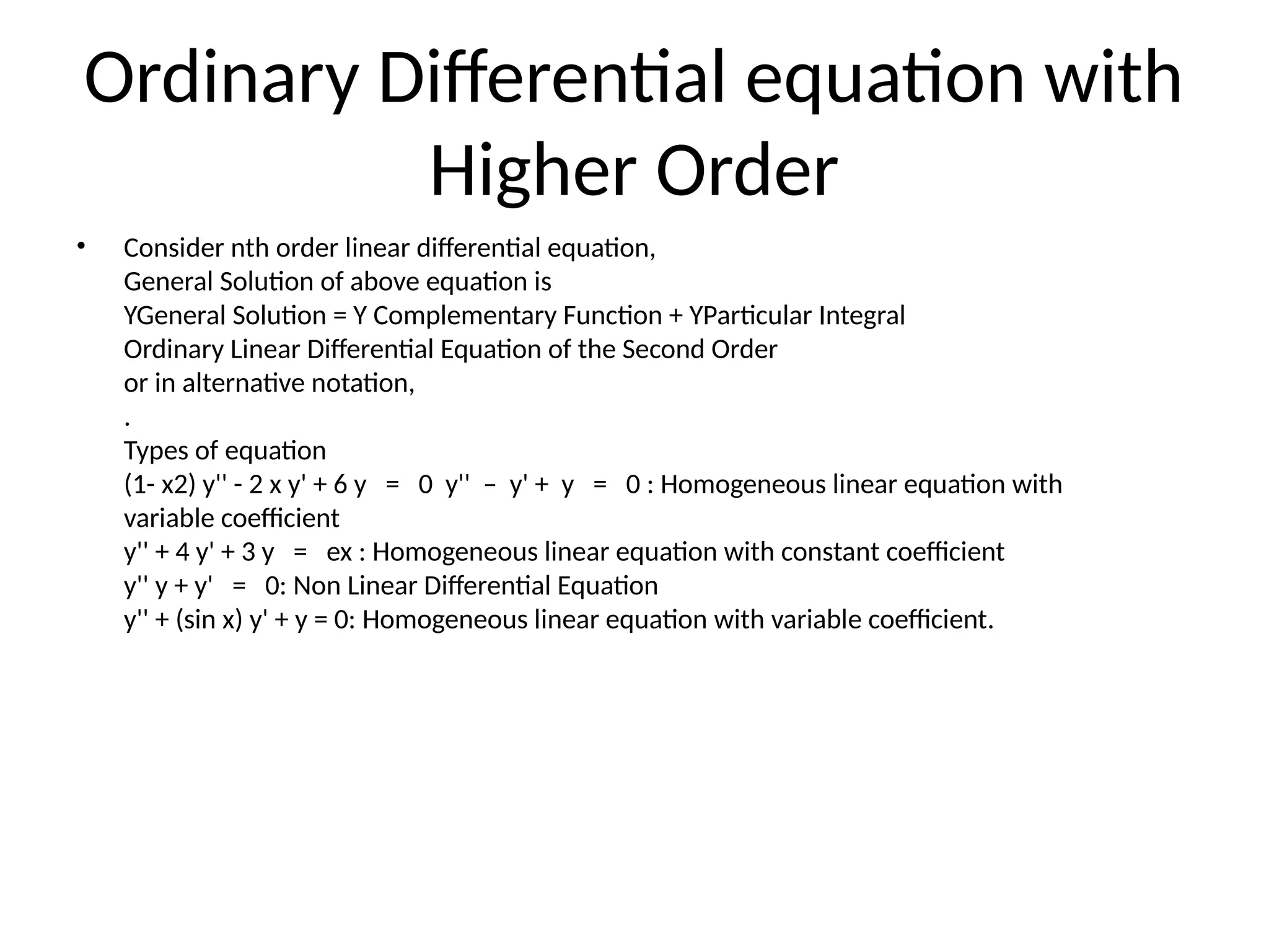
Consider nth order linear differential equation,
y^((n) ) (x)+a_1 y^((n-1) ) (x)+⋯+a_(n-1) y'(x)+a_n y(x)=r(x)
General Solution of above equation is
YGeneral Solution = Y Complementary Function + YParticular Integral
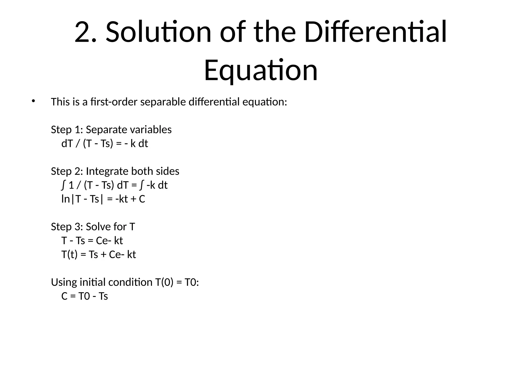
Ordinary Linear Differential Equation of the Second Order
(d^2 y)/(dx^2 )+p(x) dy/dx+q(x)y=r(x)
or in alternative notation,
y"+p(x)y^'+q(x)y=r(x).
Types of equation
(1- x2) y'' - 2 x y' + 6 y = 0 y'' – 2 x 1 - x2y' + 61 - x2y = 0 : Homogeneous linear equation with
variable coefficient
y'' + 4 y' + 3 y = ex : Homogeneous linear equation with constant coefficient
y'' y + y' = 0: Non Linear Differential Equation
y'' + (sin x) y' + y = 0: Homogeneous linear equation with variable coefficient.
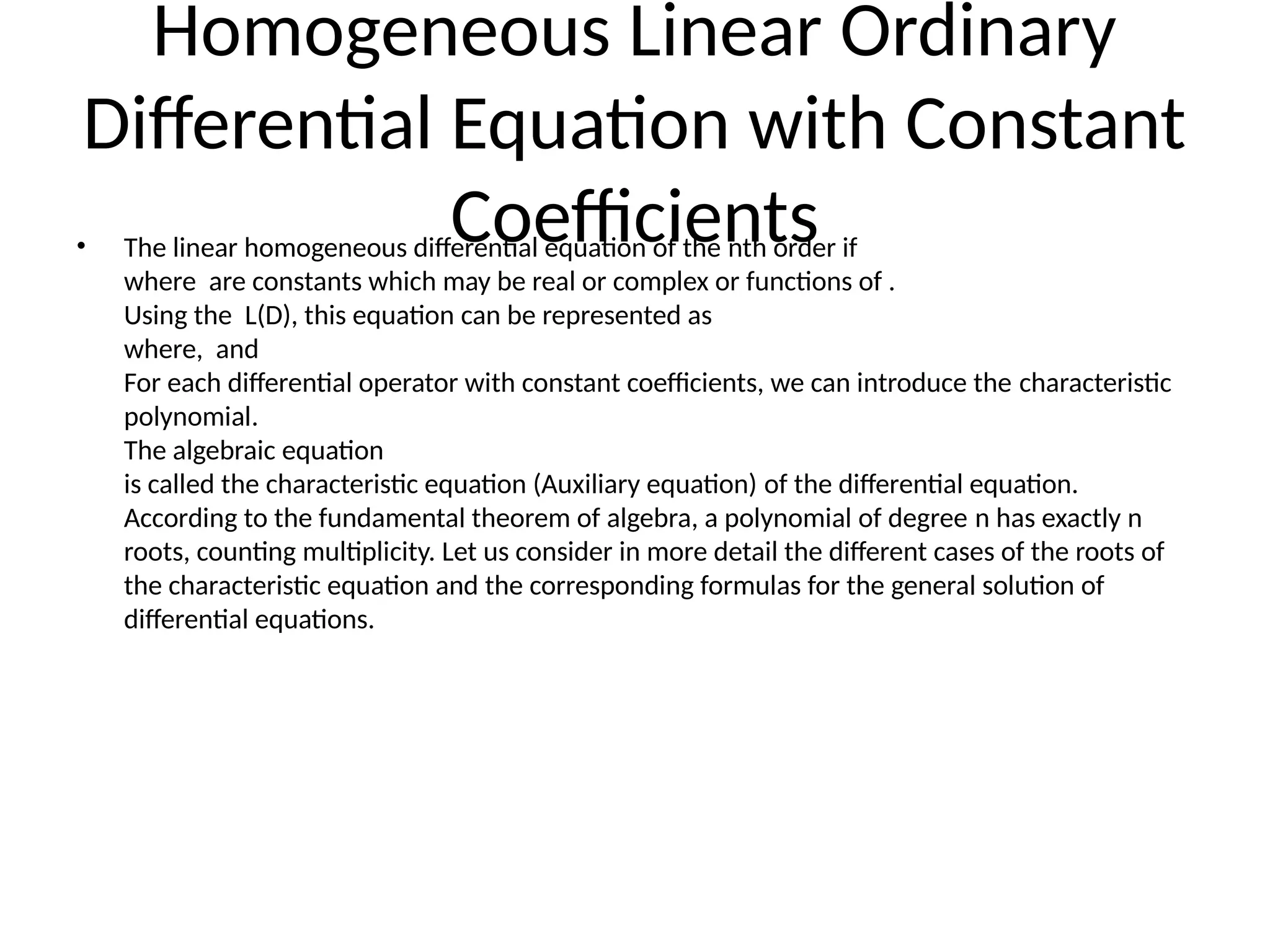
Homogeneous Linear Ordinary Differential Equation with Constant Coefficients
The linear homogeneous differential equation of the nth order if r(x)=0
y^((n)) (x)+a_1 y^((n-1)) (x)+⋯+a_(n-1) y'(x)+a_n y(x)=0,
where a_1,a_2,…,a_n are constants which may be real or complex or functions of x.
Using the linear differential operator L(D), this equation can be represented as
L(D)y(x)=0,
where, D=d/dx and L(D)=D^n+a_1 D^(n-1)+⋯+a_(n-1) D+a_n
For each differential operator with constant coefficients, we can introduce the characteristic polynomial.
L(m)=m^n+a_1 m^(n-1)+⋯+a_(n-1) m+a_n.
The algebraic equation
L(m)=m^n+a_1 m^(n-1)+⋯+a_(n-1) m+a_n.
is called the characteristic equation (Auxiliary equation) of the differential equation.
According to the fundamental theorem of algebra, a polynomial of degree n has exactly n roots, counting multiplicity. Let us consider in more detail the different cases of the roots of the characteristic equation and the corresponding formulas for the general solution of differential equations.
Case 1. All Roots of the Characteristic Equation are Real and Distinct
Assume that the characteristic equation L(m)=0 has n roots m_1,m_2,…,m_n. In this case the general solution of the differential equation is written in a simple form:
y(x)=c_1 e^(m_1 x)+c_2 e^(m_2 x)+⋯+c_n e^(m_n x),
where c_1,c_2,…,c_n are constants depending on initial conditions.
Case 2. The Roots of the Characteristic Equation are Real and Multiple
Let the characteristic equation L(m)=0 of degree n have m roots m_1,m_2,…,m_n., the multiplicity of which, respectively, is equal to m_1,m_2,…,m_nIt is clear that the following condition holds:
m_1,m_2,…,m_nThen the general solution of the homogeneous differential equations with constant coefficients has the form
y(x)=c_1 e^(m_1 x)+c_2 xe^(m_2 x)+⋯+c_k1 x^(k_1-1) e^(m_1 x)+⋯+c_n x^(km-1) e^(m_m x).
It is seen that the formula of the general solution has exactly ki terms corresponding to each root m_iof multiplicity k_i.
Case 3. The Roots of the Characteristic Equation are Complex and Distinct
If the coefficients of the differential equation are real numbers, the complex roots of the characteristic equation will be presented in the form of conjugate pairs of complex numbers:


![Week 8 [compatibility mode]](https://cdn.slidesharecdn.com/ss_thumbnails/week8compatibilitymode-130213163443-phpapp01-thumbnail.jpg?width=640&height=640&fit=bounds)


