Bayes’ rule
Let B1, B2,...., Bn be the set of ‘n’ mutually exclusive and exhaustive events,
whose union is the random sample space of an experiment. If A be any arbitrary
event of the sample space of the above experiment with P(A) ≠0, then the
probability of the event B has actually occurred is given by P(Bi/A), where
P(Bi/A) = P (A&B)/ [P(A & B1) + P(A & B2) + ............+ P(A & Bn) ]
Bayes’ Rule: derivation
)
(
)
&
(
)
/
(
B
P
B
A
P
B
A
P 
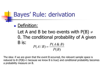
 Definition:
Let A and B be two events with P(B) 
0. The conditional probability of A given
B is:
The idea: if we are given that the event B occurred, the relevant sample space is
reduced to B {P(B)=1 because we know B is true} and conditional probability becomes
a probability measure on B.
Bayes’ Rule: derivation
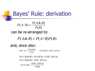
can be re-arranged to:
)
(
)
/
(
)
&
( B
P
B
A
P
B
A
P 
)
(
)
/
(
)
&
(
)
(
)
&
(
)
/
( A
P
A
B
P
B
A
P
A
P
B
A
P
A
B
P 


)
(
)
(
)
/
(
)
/
(
)
(
)
/
(
)
(
)
/
(
)
(
)
/
(
)
&
(
)
(
)
/
(
B
P
A
P
A
B
P
B
A
P
A
P
A
B
P
B
P
B
A
P
A
P
A
B
P
B
A
P
B
P
B
A
P





)
(
)
&
(
)
/
(
B
P
B
A
P
B
A
P 
and, since also:
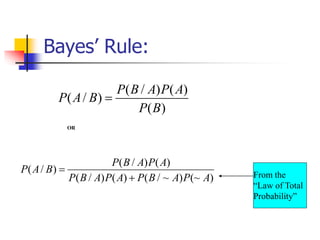
Bayes’ Rule:
)
(
)
(
)
/
(
)
/
(
B
P
A
P
A
B
P
B
A
P 
From the
“Law of Total
Probability”
OR
)
(~
)
~
/
(
)
(
)
/
(
)
(
)
/
(
)
/
(
A
P
A
B
P
A
P
A
B
P
A
P
A
B
P
B
A
P


Bayes’ Rule:
 Why do we care??
 Why is Bayes’ Rule useful??
 It turns out that sometimes it is very
useful to be able to “flip” conditional
probabilities. That is, we may know the
probability of A given B, but the
probability of B given A may not be
obvious. An example will help…
In-Class Exercise
 If HIV has a prevalence of 3% in San
Francisco, and a particular HIV test has a
false positive rate of .001 and a false
negative rate of .01, what is the probability
that a random person who tests positive is
actually infected (also known as “positive
predictive value”)?
Answer: using probability tree
______________
1.0
P(test +)=.99
P(+)=.03
P(-)=.97
P(test - = .01)
P(test +) = .001
P (+, test +)=.0297
P(+, test -)=.003
P(-, test +)=.00097
P(-, test -) = .96903
P(test -) = .999
A positive test places one on either of the two “test +” branches.
But only the top branch also fulfills the event “true infection.”
Therefore, the probability of being infected is the probability of being on the top
branch given that you are on one of the two circled branches above.
%
8
.
96
00097
.
0297
.
0297
.
)
(
)
&
(
)
/
( 








test
P
true
test
P
test
P
Answer: using Bayes’ rule
%
8
.
96
)
97
(.
001
.
)
03
(.
99
.
)
03
(.
99
.
)
(
)
/
(
)
(
)
/
(
)
(
)
/
(
)
/
(
















true
P
true
test
P
true
P
true
test
P
true
P
true
test
P
test
true
P
Conditional Probability for
Epidemiology:
The odds ratio and risk ratio
as conditional probability
The Risk Ratio and the Odds
Ratio as conditional probability
In epidemiology, the association between a
risk factor or protective factor (exposure) and
a disease may be evaluated by the “risk ratio”
(RR) or the “odds ratio” (OR).
Both are measures of “relative risk”—the
general concept of comparing disease risks in
exposed vs. unexposed individuals.
Odds and Risk (probability)
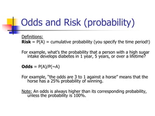
Definitions:
Risk = P(A) = cumulative probability (you specify the time period!)
For example, what’s the probability that a person with a high sugar
intake develops diabetes in 1 year, 5 years, or over a lifetime?
Odds = P(A)/P(~A)
For example, “the odds are 3 to 1 against a horse” means that the
horse has a 25% probability of winning.
Note: An odds is always higher than its corresponding probability,
unless the probability is 100%.
Odds vs. Risk=probability
If the risk is… Then the odds
are…
½ (50%)
¾ (75%)
1/10 (10%)
1/100 (1%)
Note: An odds is always higher than its corresponding probability,
unless the probability is 100%.
1:1
3:1
1:9
1:99
Cohort Studies (risk ratio)
Target
population
Exposed
Not
Exposed
Disease-free
cohort
Disease
Disease-free
Disease
Disease-free
TIME
Exposure (E) No Exposure
(~E)
Disease (D) a b
No Disease (~D) c d
a+c b+d
)
/(
)
/(
)
~
/
(
)
/
(
d
b
b
c
a
a
E
D
P
E
D
P
RR




risk to the exposed
risk to the unexposed
The Risk Ratio
400 400
1100 2600
0
.
2
3000
/
400
1500
/
400 

RR
Hypothetical Data
Normal BP
Congestive
Heart Failure
No CHF
1500 3000
High Systolic BP
Target
population
Exposed in
past
Not exposed
Exposed
Not Exposed
Case-Control Studies (odds
ratio)
Disease
(Cases)
No Disease
(Controls)
bc
ad
d
c
b
a
OR
D
E
P
D
E
P
D
E
P
D
E
P



)
~
/
(~
)
~
/
(
)
/
(~
)
/
(
Exposure (E) No Exposure
(~E)
Disease (D) a b
No Disease (~D) c d
The Odds Ratio (OR)
Odds of exposure
in the cases
Odds of exposure
in the controls
The Odds Ratio (OR)
Odds of disease in
the exposed
Odds of disease in
the unexposed
)
~
/
(~
)
~
/
(
)
/
(~
)
/
(
D
E
P
D
E
P
D
E
P
D
E
P
OR 
Odds of exposure
in the cases
Odds of exposure
in the controls
)
~
/
(~
)
~
/
(
)
/
(~
)
/
(
E
D
P
E
D
P
E
D
P
E
D
P
But, this
expression is
mathematically
equivalent to:
Backward from what we
want…
The direction of interest!
Interpretation of the odds
ratio:
 The odds ratio will always be bigger
than the corresponding risk ratio if RR
>1 and smaller if RR <1 (the harmful or
protective effect always appears larger)
 The magnitude of the inflation depends
on the prevalence of the disease.
The rare disease assumption
RR
OR E
D
P
E
D
P
E
D
P
E
D
P
E
D
P
E
D
P


 )
~
/
(
)
/
(
)
~
/
(~
)
~
/
(
)
/
(~
)
/
(
1
1
When a disease is rare:
P(~D) = 1 - P(D)  1
The odds ratio vs. the risk ratio
1.0 (null)
Odds ratio
Risk ratio Risk ratio
Odds ratio
Odds ratio
Risk ratio Risk ratio
Odds ratio
Rare Outcome
Common Outcome
1.0 (null)
Interpreting ORs when the
outcome is common…
 If the outcome has a 10% prevalence in the
unexposed/reference group*, the maximum possible
RR=10.0.
 For 20% prevalence, the maximum possible RR=5.0
 For 30% prevalence, the maximum possible RR=3.3.
 For 40% prevalence, maximum possible RR=2.5.
 For 50% prevalence, maximum possible RR=2.0.
*Authors should report the prevalence/risk of the outcome in the
unexposed/reference group, but they often don’t. If this number is not given,
you can usually estimate it from other data in the paper (or, if it’s important
enough, email the authors).
Interpreting ORs when the
outcome is common…
Formula from: Zhang J. What's the Relative Risk? A Method of Correcting the Odds
Ratio in Cohort Studies of Common Outcomes JAMA. 1998;280:1690-1691.
)
(
)
1
( OR
P
P
OR
RR
o
o 



Where:
OR = odds ratio from logistic regression (e.g., 3.92)
P0 = P(D/~E) = probability/prevalence of the outcome in the
unexposed/reference group (e.g. ~45%)
If data are from a cross-sectional or cohort study, then you can
convert ORs (from logistic regression) back to RRs with a simple
formula:

Understanding the conditional probability

  • 1.
    Bayes’ rule Let B1,B2,...., Bn be the set of ‘n’ mutually exclusive and exhaustive events, whose union is the random sample space of an experiment. If A be any arbitrary event of the sample space of the above experiment with P(A) ≠0, then the probability of the event B has actually occurred is given by P(Bi/A), where P(Bi/A) = P (A&B)/ [P(A & B1) + P(A & B2) + ............+ P(A & Bn) ]
  • 2.
    Bayes’ Rule: derivation ) ( ) & ( ) / ( B P B A P B A P  Definition: Let A and B be two events with P(B)  0. The conditional probability of A given B is: The idea: if we are given that the event B occurred, the relevant sample space is reduced to B {P(B)=1 because we know B is true} and conditional probability becomes a probability measure on B.
  • 3.
    Bayes’ Rule: derivation canbe re-arranged to: ) ( ) / ( ) & ( B P B A P B A P  ) ( ) / ( ) & ( ) ( ) & ( ) / ( A P A B P B A P A P B A P A B P    ) ( ) ( ) / ( ) / ( ) ( ) / ( ) ( ) / ( ) ( ) / ( ) & ( ) ( ) / ( B P A P A B P B A P A P A B P B P B A P A P A B P B A P B P B A P      ) ( ) & ( ) / ( B P B A P B A P  and, since also:
  • 4.
    Bayes’ Rule: ) ( ) ( ) / ( ) / ( B P A P A B P B A P  Fromthe “Law of Total Probability” OR ) (~ ) ~ / ( ) ( ) / ( ) ( ) / ( ) / ( A P A B P A P A B P A P A B P B A P  
  • 5.
    Bayes’ Rule:  Whydo we care??  Why is Bayes’ Rule useful??  It turns out that sometimes it is very useful to be able to “flip” conditional probabilities. That is, we may know the probability of A given B, but the probability of B given A may not be obvious. An example will help…
  • 6.
    In-Class Exercise  IfHIV has a prevalence of 3% in San Francisco, and a particular HIV test has a false positive rate of .001 and a false negative rate of .01, what is the probability that a random person who tests positive is actually infected (also known as “positive predictive value”)?
  • 7.
    Answer: using probabilitytree ______________ 1.0 P(test +)=.99 P(+)=.03 P(-)=.97 P(test - = .01) P(test +) = .001 P (+, test +)=.0297 P(+, test -)=.003 P(-, test +)=.00097 P(-, test -) = .96903 P(test -) = .999 A positive test places one on either of the two “test +” branches. But only the top branch also fulfills the event “true infection.” Therefore, the probability of being infected is the probability of being on the top branch given that you are on one of the two circled branches above. % 8 . 96 00097 . 0297 . 0297 . ) ( ) & ( ) / (          test P true test P test P
  • 8.
    Answer: using Bayes’rule % 8 . 96 ) 97 (. 001 . ) 03 (. 99 . ) 03 (. 99 . ) ( ) / ( ) ( ) / ( ) ( ) / ( ) / (                 true P true test P true P true test P true P true test P test true P
  • 9.
    Conditional Probability for Epidemiology: Theodds ratio and risk ratio as conditional probability
  • 10.
    The Risk Ratioand the Odds Ratio as conditional probability In epidemiology, the association between a risk factor or protective factor (exposure) and a disease may be evaluated by the “risk ratio” (RR) or the “odds ratio” (OR). Both are measures of “relative risk”—the general concept of comparing disease risks in exposed vs. unexposed individuals.
  • 11.
    Odds and Risk(probability) Definitions: Risk = P(A) = cumulative probability (you specify the time period!) For example, what’s the probability that a person with a high sugar intake develops diabetes in 1 year, 5 years, or over a lifetime? Odds = P(A)/P(~A) For example, “the odds are 3 to 1 against a horse” means that the horse has a 25% probability of winning. Note: An odds is always higher than its corresponding probability, unless the probability is 100%.
  • 12.
    Odds vs. Risk=probability Ifthe risk is… Then the odds are… ½ (50%) ¾ (75%) 1/10 (10%) 1/100 (1%) Note: An odds is always higher than its corresponding probability, unless the probability is 100%. 1:1 3:1 1:9 1:99
  • 13.
    Cohort Studies (riskratio) Target population Exposed Not Exposed Disease-free cohort Disease Disease-free Disease Disease-free TIME
  • 14.
    Exposure (E) NoExposure (~E) Disease (D) a b No Disease (~D) c d a+c b+d ) /( ) /( ) ~ / ( ) / ( d b b c a a E D P E D P RR     risk to the exposed risk to the unexposed The Risk Ratio
  • 15.
    400 400 1100 2600 0 . 2 3000 / 400 1500 / 400  RR Hypothetical Data Normal BP Congestive Heart Failure No CHF 1500 3000 High Systolic BP
  • 16.
    Target population Exposed in past Not exposed Exposed NotExposed Case-Control Studies (odds ratio) Disease (Cases) No Disease (Controls)
  • 17.
    bc ad d c b a OR D E P D E P D E P D E P    ) ~ / (~ ) ~ / ( ) / (~ ) / ( Exposure (E) NoExposure (~E) Disease (D) a b No Disease (~D) c d The Odds Ratio (OR) Odds of exposure in the cases Odds of exposure in the controls
  • 18.
    The Odds Ratio(OR) Odds of disease in the exposed Odds of disease in the unexposed ) ~ / (~ ) ~ / ( ) / (~ ) / ( D E P D E P D E P D E P OR  Odds of exposure in the cases Odds of exposure in the controls ) ~ / (~ ) ~ / ( ) / (~ ) / ( E D P E D P E D P E D P But, this expression is mathematically equivalent to: Backward from what we want… The direction of interest!
  • 19.
    Interpretation of theodds ratio:  The odds ratio will always be bigger than the corresponding risk ratio if RR >1 and smaller if RR <1 (the harmful or protective effect always appears larger)  The magnitude of the inflation depends on the prevalence of the disease.
  • 20.
    The rare diseaseassumption RR OR E D P E D P E D P E D P E D P E D P    ) ~ / ( ) / ( ) ~ / (~ ) ~ / ( ) / (~ ) / ( 1 1 When a disease is rare: P(~D) = 1 - P(D)  1
  • 21.
    The odds ratiovs. the risk ratio 1.0 (null) Odds ratio Risk ratio Risk ratio Odds ratio Odds ratio Risk ratio Risk ratio Odds ratio Rare Outcome Common Outcome 1.0 (null)
  • 22.
    Interpreting ORs whenthe outcome is common…  If the outcome has a 10% prevalence in the unexposed/reference group*, the maximum possible RR=10.0.  For 20% prevalence, the maximum possible RR=5.0  For 30% prevalence, the maximum possible RR=3.3.  For 40% prevalence, maximum possible RR=2.5.  For 50% prevalence, maximum possible RR=2.0. *Authors should report the prevalence/risk of the outcome in the unexposed/reference group, but they often don’t. If this number is not given, you can usually estimate it from other data in the paper (or, if it’s important enough, email the authors).
  • 23.
    Interpreting ORs whenthe outcome is common… Formula from: Zhang J. What's the Relative Risk? A Method of Correcting the Odds Ratio in Cohort Studies of Common Outcomes JAMA. 1998;280:1690-1691. ) ( ) 1 ( OR P P OR RR o o     Where: OR = odds ratio from logistic regression (e.g., 3.92) P0 = P(D/~E) = probability/prevalence of the outcome in the unexposed/reference group (e.g. ~45%) If data are from a cross-sectional or cohort study, then you can convert ORs (from logistic regression) back to RRs with a simple formula: