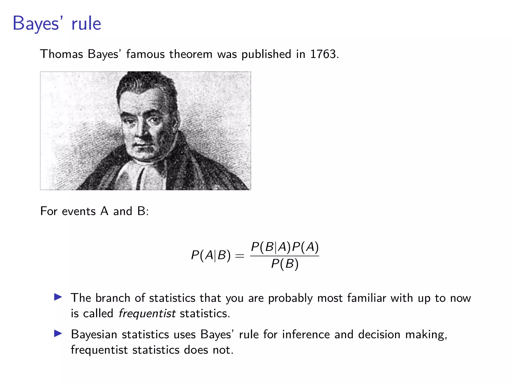
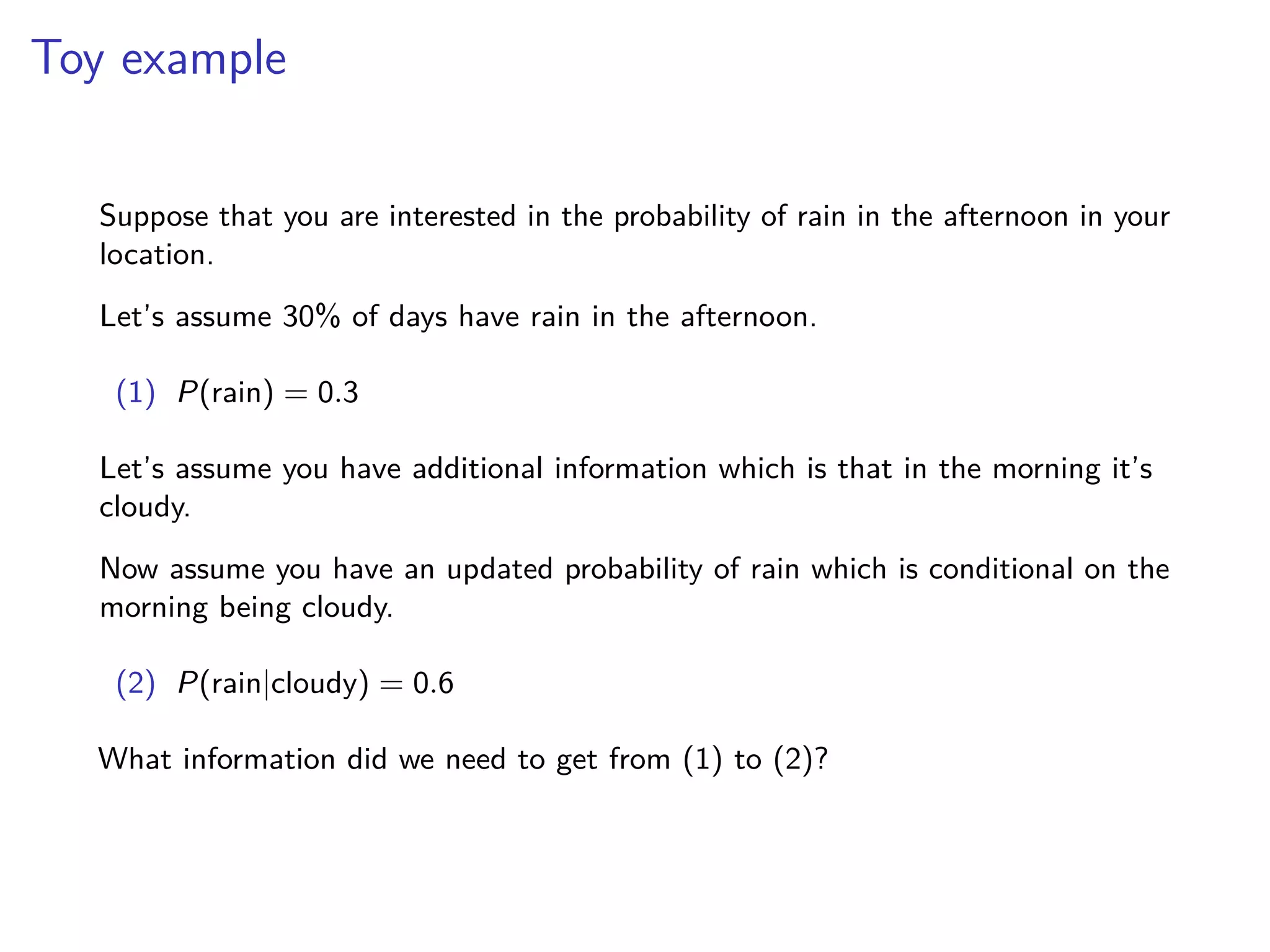
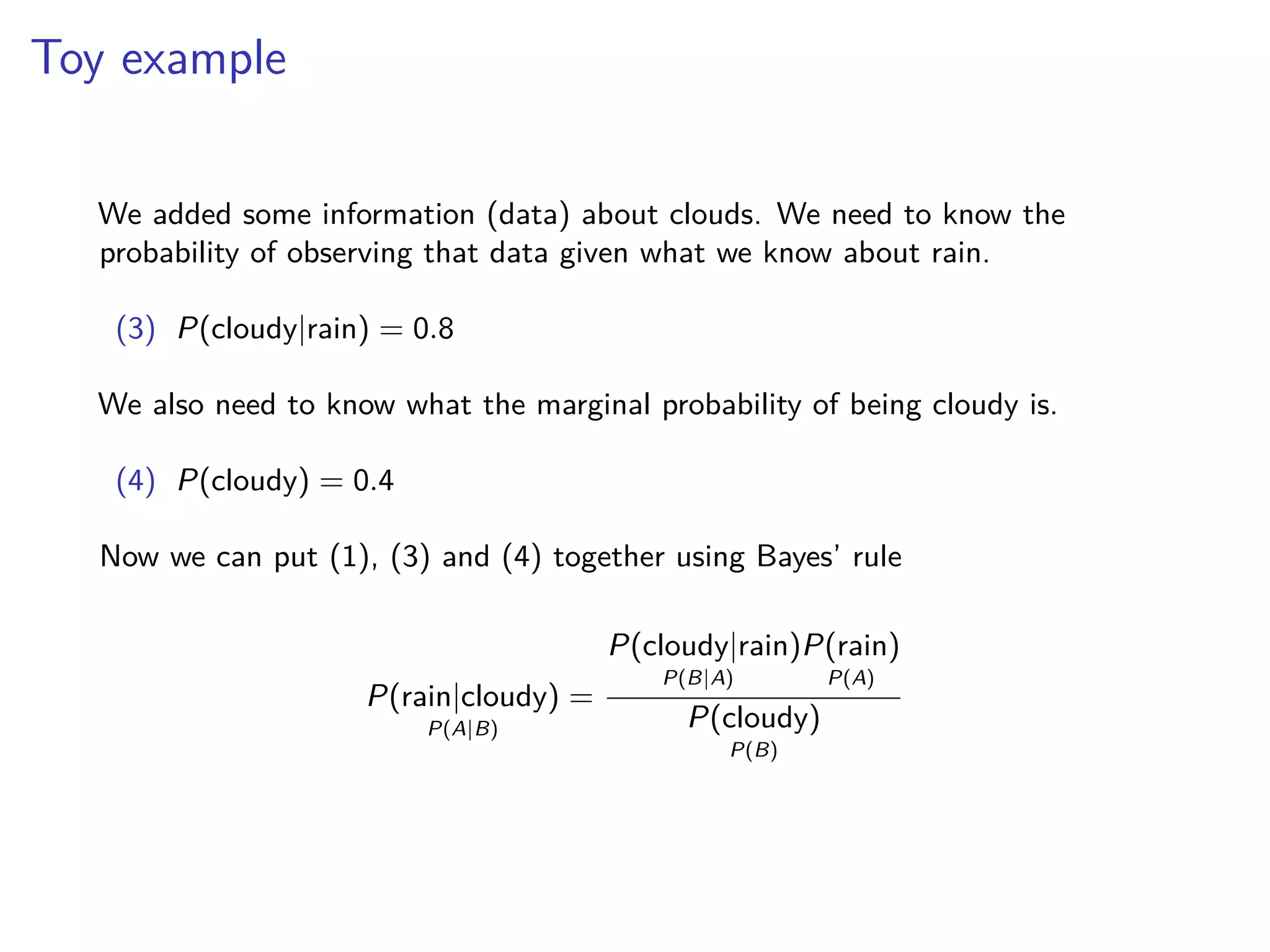
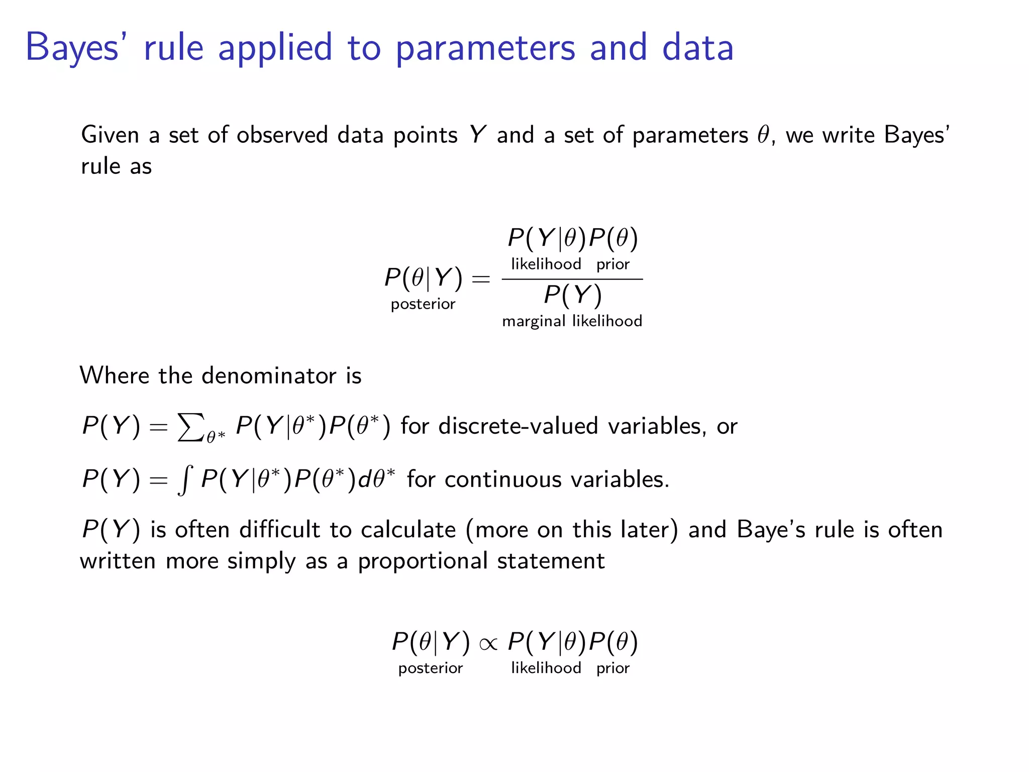
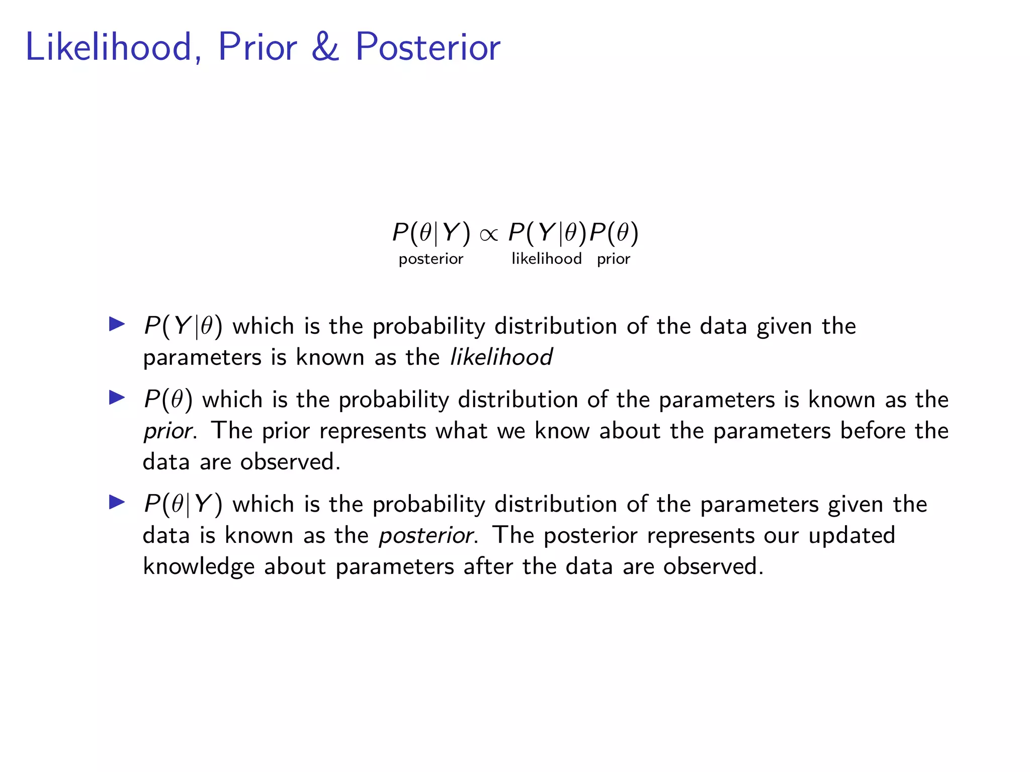
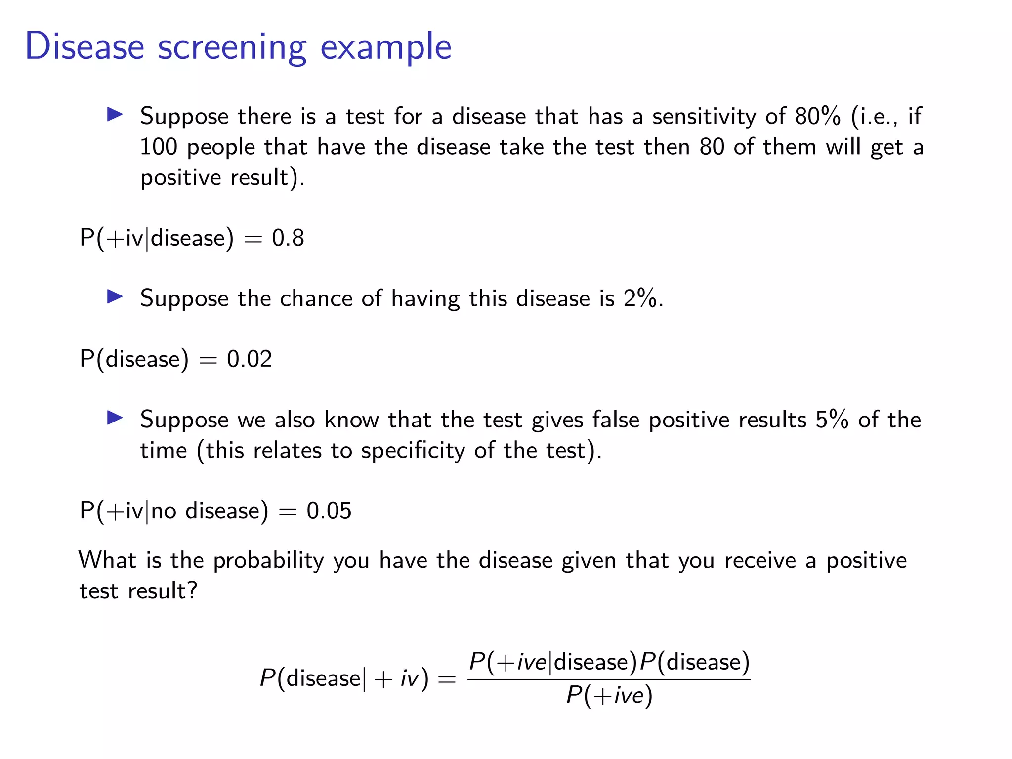
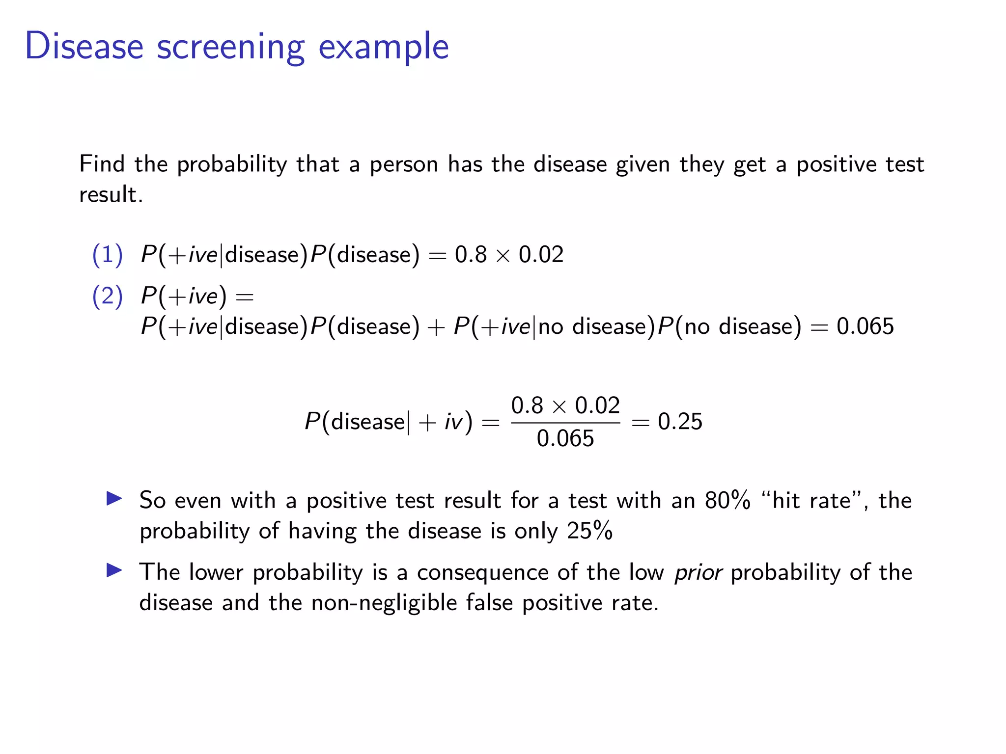
1) Bayesian statistics uses Bayes' rule for inference and decision making, while frequentist statistics does not. 2) Bayes' rule allows you to calculate the probability of an event given additional information, such as calculating the probability of rain given that it is cloudy in the morning. 3) Even with a positive test result, the probability of having a disease can be low due to the low prior probability of the disease and potential for false positives.

1. Bayesian Data Analysis
Dr Niamh Cahill (she/her)
Bayes’ Rule

2. Bayes’ rule
Thomas Bayes’ famous theorem was published in 1763.
For events A and B:
P(A|B) =
P(B|A)P(A)
P(B)
▶ The branch of statistics that you are probably most familiar with up to now
is called frequentist statistics.
▶ Bayesian statistics uses Bayes’ rule for inference and decision making,
frequentist statistics does not.

3. Toy example
Suppose that you are interested in the probability of rain in the afternoon in your
location.
Let’s assume 30% of days have rain in the afternoon.
(1) P(rain) = 0.3
Let’s assume you have additional information which is that in the morning it’s
cloudy.
Now assume you have an updated probability of rain which is conditional on the
morning being cloudy.
(2) P(rain|cloudy) = 0.6
What information did we need to get from (1) to (2)?

4. Toy example
We added some information (data) about clouds. We need to know the
probability of observing that data given what we know about rain.
(3) P(cloudy|rain) = 0.8
We also need to know what the marginal probability of being cloudy is.
(4) P(cloudy) = 0.4
Now we can put (1), (3) and (4) together using Bayes’ rule
P(rain|cloudy)
P(A|B)
=
P(cloudy|rain
P(B|A)
)P(rain)
P(A)
P(cloudy)
P(B)

5. Disease screening example
▶ Suppose there is a test for a disease that has a sensitivity of 80% (i.e., if
100 people that have the disease take the test then 80 of them will get a
positive result).
P(+iv|disease) = 0.8
▶ Suppose the chance of having this disease is 2%.
P(disease) = 0.02
▶ Suppose we also know that the test gives false positive results 5% of the
time (this relates to specificity of the test).
P(+iv|no disease) = 0.05
What is the probability you have the disease given that you receive a positive
test result?
P(disease| + iv) =
P(+ive|disease)P(disease)
P(+ive)

6. Disease screening example
Find the probability that a person has the disease given they get a positive test
result.
(1) P(+ive|disease)P(disease) = 0.8 × 0.02
(2) P(+ive) =
P(+ive|disease)P(disease) + P(+ive|no disease)P(no disease) = 0.065
P(disease| + iv) =
0.8 × 0.02
0.065
= 0.25
▶ So even with a positive test result for a test with an 80% “hit rate”, the
probability of having the disease is only 25%
▶ The lower probability is a consequence of the low prior probability of the
disease and the non-negligible false positive rate.

7. Bayes’ rule applied to parameters and data
Given a set of observed data points Y and a set of parameters θ, we write Bayes’
rule as
P(θ|Y )
posterior
=
P(Y |θ)
likelihood
P(θ)
prior
P(Y )
marginal likelihood
Where the denominator is
P(Y ) =
P
θ∗ P(Y |θ∗
)P(θ∗
) for discrete-valued variables, or
P(Y ) =
R
P(Y |θ∗
)P(θ∗
)dθ∗
for continuous variables.
P(Y ) is often difficult to calculate (more on this later) and Baye’s rule is often
written more simply as a proportional statement
P(θ|Y )
posterior
∝ P(Y |θ)
likelihood
P(θ)
prior

8. Likelihood, Prior & Posterior
P(θ|Y )
posterior
∝ P(Y |θ)
likelihood
P(θ)
prior
▶ P(Y |θ) which is the probability distribution of the data given the
parameters is known as the likelihood
▶ P(θ) which is the probability distribution of the parameters is known as the
prior. The prior represents what we know about the parameters before the
data are observed.
▶ P(θ|Y ) which is the probability distribution of the parameters given the
data is known as the posterior. The posterior represents our updated
knowledge about parameters after the data are observed.