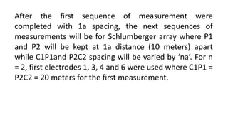
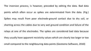
This document provides an introduction and outline for a study on using two-dimensional electrical resistivity imaging to classify lithology in the subsurface of Ujemen, Nigeria. It discusses how electrical resistivity tomography can produce high-resolution images of subsurface layers. The methodology section describes how resistivity is measured using different electrode configurations based on Ohm's law. Previous related works that used electrical resistivity to investigate geology and groundwater in Nigeria are also summarized.

1. TWO DIMENSIONAL ELECTRICAL RESISTIVITY IMAGING SURVEY
FOR LITHOSTRATIGRAPHIC CLASSIFICATION OF THE
SUBSURFACE, UJEMEN, EKPOMA-NIGERIA
BY
AIREWELE Ehizokhale
(B.Sc., M.Sc. Exploration Geophysics)
SUPERVISOR:
PROF. O.M. ALILIE

2. OUTLINE OF PRESENTATION
INTRODUCTION
 Background to the study
 Statement of the Problem
 Justification of Research
 Study Area
 Aim and Objectives
 METHODOLOGY
 RESULTS AND DISCUSSION
CONCLUSION
 RECOMMENDATION
CONTRIBUTION TO KNOWLEDGE
REFERENCES

3. INTRODUCTION
Background to the study
Over the years, humans have explored the effect of subsurface
structures, such as zone of weakness on geotechnical and engineering
structures which has led to the development of geophysical methods
for subsurface classification in area of complex geology.
(Mwenifumbo, 1997; Pellerin, 2002; Osazuwa and Abdullahi, 2008;
Osazuwa and Chii, 2010; Ayolabi et al., 2012, 2013; Venkateswarlu et
al., 2014; Aminu, 2015).
Many geophysical methods are available, with each of these methods
having its own advantages and disadvantages depending on the
target study area (Aizebeokhai, 2010).

4. In the last few decades, the development of multi-electrode
arrays, automated acquisition systems, and new inversion
algorithms used for Electrical Resistivity Tomography (ERT) have
renewed researchers’ interests in electrical methods. The method
has emerged recently as an alternative technique to investigate
and classify the subsurface at various scales where the use of
conventional resistivity techniques is unsuitable in complex
geological area. (Griffiths and Baker, 1993; Loke and Barker, 1996;
2000, 2004).

5. Examples of geophysical techniques are the two-
dimensional and three-dimensional geo-electrical
resistivity imaging methods. With the new advancement,
subsurface characteristics is revealed which enhance
understanding of subsurface geologic condition.

6. In Electrical Resistivity Tomography method, the sounding and
profiling techniques are integrated to give information on the
lateral and vertical extent of the surface. The Electrical
Resistivity Tomography gives images either in two-
dimensional or three-dimensional depending on how the data
was acquired.
As a result of the availability of automated data acquisition
systems and efficient user friendly inversion software,
Electrical Resistivity Tomography is popular nowadays due its
ability to produce images of the subsurface efficiently and
effectively.

7. Geophysical survey of subsurface involves the measurement of
geoelectric parameters such as layer resistivity (ρa), thickness and
depth for each lithological unit, geoelectric parameters can as well be
used to describe the hydrological condition of the subsurface. To
effectively map and characterize unit within the subsurface, the
knowledge of the various lithological units, their distribution and
characteristics must be put into consideration (Zohdy, 1965).
Different electrode configuration can be use to conduct electrical
resistivity survey, which includes Wenner array, Schlumberger array,
dipole-dipole, pole-dipole, pole-pole, square and gradient arrays.

8. The Electrical Resistivity Tomography method has been extensively used in a number of
near surface exploration since the first usage around 1830 (Parasins 1962). They include
groundwater exploration (Ayolabi et al., 2009), mapping subsurface structures (Khalil
2009), geotechnical and engineering site investigation (Giao et al., 2010; Folorunso et
al.,2012), exploration and evaluation of ore deposit (Ramazi et al., 2009), mapping of
soil and groundwater contamination (Cahyna et al., 1990), groundwater quality
assessment (Ayolabi et al., 2009), as well as geological discontinuities such as faults,
drainage channel systems and other structures features (Lebourg et al., 2005) and
surface structure failure (Egwuonwu et al., 2011).

9. Problem Statement.
Previous work carried out within and around the area of study (AAU main
campus) employed the one-Dimensional (VES) technique for water potential
zones investigation and subsurface studies. A more accurate model of the
subsurface will be a 2-Dimensional Electrical Resistivity model where
resistivity changes in the vertical direction as well as in the horizontal
direction along the survey line which was adopted for this research.

10. Justification of the Research
Mondal et al., (2008) demonstrated that electrical resistivity imaging (ERI) method can give
a better picture of the concealed structures, than the conventional maps of true resistivity
contours using the vertical electrical sounding method.
Due to the limitations of the conventional resistivity sounding and profiling, two
dimensional electrical resistivity imaging was used in this study for mapping the subsurface
layers because it’s capable of yielding adequate information on subsurface rock types and
distribution.

11. STUDY AREA.
The study area, Ujemen community is located along the Benin-Auchi
express road in Esan West Local Government of Edo State. It lies
between Latitude 6◦44’38.32”N and longitude 6◦5’2.71”E. The area
lies within the tropical region.
The area falls within the Southwestern Sedimentary terrain of Nigeria.
The rocks in the area are of ages between Paleocene to recent. (Alile et
al; 2011). The Sedimentary rocks in the area contains 90% of
sandstone and shale intercalation

14. Previous Works on Subsurface Classification
Alile et al., (2010) carried out a geoelectric investigation for ground water in
Obaretin-lyanomon locality, Edo State, Nigeria. Their findings provided
information on the depth to the ground water and probable the thickness of
the aquifer unit in the study area. Both vertical electrical sounding and
borehole data were used in delineating the geo electric sections. Their findings
reveal a correlation between vertical electrical sounding and the borehole data

15. Bayewu et al, (2012) delineated the anon-conformity around Ijesha-Ijebu,
Southern western, Nigeria using Electrical Resistivity Imaging (ERI). Using
Wenner’s array they probed a total of five to six levels for the traverse. With
this they were able to cover a distance of 0.5 to Ikm. Also, they used inversion
method to acquire the pseudosection using DIPRO software. From the
lithological section of the area produced they found a conglometric layer of 5-
10m thick lying conformably on the banded gneiss.

16. The lithology also revealed a top soil sandy layer of 0.8-2m with a
ferruginous sandstone of 7-10m in thickness below it. Also the Electrical
Resistivity Imaging also revealed three geoelectric layers namely; a sandy
topsoil with a resistivity of 500-1300Ωm, a highly resistive conglomerate
layer with resistivity of >1350Ωm and lastly a weathered basement rock
with resistivity of 400 - 1350Ωm.

17. Oyeyemi and Olofinade (2016) embarked on a geoelectrical-geotechnical
studies for the near surface characterization of Lekki-Epe, Lagos, Nigeria.
The aim of the research was to characterize the near surface materials by
using both geoelectric resistivity tomography and geotechnical techniques
with a view to unravelling the foundational failures witnessed in the
country. Using Wenners array, four traverses of the geoelectrical resistivity
were was conducted. Also, a cone penetrating data was also obtained
along the same traverse. From the results obtained, three different
lithogies where delineated. These include loose sand (50 -260Ωm),
compacted clayey sand (20 – 72.2Ωm) and clay/peat (˂27.5Ωm)
respectively.

18. Salafu and Ujuanbi (2015) worked on identifying occurrence of
deformational structures in Esan part of Anambra basin. From their
findings, integrated study (geological & geophysical) shows the occurrence
of deformational structure (faults &folds). They concluded that the
deformational structures are potential hydrocarbon traps and they control
the hydrologic settings of Esan land.

19. THEORY AND METHODOLOGY
The resistivity method is based on the principles of Ohm’s law. In 1872,
George Simon Ohm derived empirical relationship between the resistance
(R) of a resistor in a simple series circuit, the current passing through the
resistor (I) and the corresponding change is potential (AV)
∆𝑣 = 𝐼𝑅 (1)

20. The electrical resistivity tomography is based on this relationship (Equation 1)
which combines the electrical, I, resistance, R, and potential difference, V,
across the conductor by considering a single current electrode (Figure ) on the
surface of a medium of uniform resistivity using the array configuration
(Figure ) (Kearey et al., 2002; Gibson and George, 2003).

23. Consider a continuous current injected into the ground through the
current electrodes (C1 & C2) as shown in fig (), the potential (∆𝑉) at
the centre will be the algebraic sum of the potentials due to
current source electrode at point A and the current sink electrode
at point B.

24. The potential difference measured at M is given as
𝑉𝑚 =
𝜌𝑙
2𝜋
1
𝑟𝐴
−
1
𝑟𝐵
(2)
Similarly, the resultant potential at N is
𝑉𝑛 =
𝜌𝑙
2𝜋
1
𝑅𝐴
−
1
𝑅𝐵
(3)

25. The potential difference measured by the voltmeter connected between M & N is given as
∆𝑉 =
𝜌𝑙
2𝜋
1
𝑟𝐴
−
1
𝑟𝐵
−
1
𝑅𝐴
−
𝐼
𝑅𝐵
(4)
Therefore,
𝜌𝑎 =
2𝜋∆𝑣
𝐼
1
𝑟𝐴
−
1
𝑟𝐵
−
1
𝑅𝐴
−
1
𝑅𝐵
− 1 (5)
Where
∆𝑉
𝐼
is the resistance of the ground measured in Ohms. Equation (5) is the basic equation
for calculating apparent resistivity. (Keary and Brooks, 1991)

26. 𝜌𝑎 =
𝑘∆𝑉
𝐼
(6)
Where
𝑘 =
2𝜋
1
𝑟𝐴
−
1
𝑟𝐵
−
1
𝑅𝐴
−
1
𝑅𝐵
(7)
The apparent resistivity 𝜌𝑎 is therefore expressed as equation (6) measured
in ohm-m (Ωm) and k is called the geometric factor of the electrode
arrangement.

27. TYPES OF ARRAY CONFIGURATION.
The manner in which electrodes are positioned relative
to one-another is known as the array type. (Figure ). In
practice, array types commonly used are: Wenner,
Schlumberger, Dipole-dipole, Gradient, pole-pole, pole-
dipole and squared array (Loke, 2002, 2004). The choice
of the array for a field work depends on the structure to
be investigated, the sensitivity of the instrument and
background noise level. (Loke, 2009).

28. Others are: depth of investigation, sensitivity of the
array to vertical and horizontal changes in the
subsurface resistivity, horizontal data coverage and
time. In each configuration, the four electrodes are
kept in a line, but their geometries and spacing are
different. (Lowrie, 1997). The value of the apparent
resistivity depends on the geometry of electrodes
used. (K factor).

31. Field Data Acquisition Procedures/Measurement
The geophysical investigation was conducted on the second week of October,
2018, during the rainy season period. The field employs the use of Pasi Earth
Resistivity meter (16-GL), two sets of 100m cable reels, P-100N
Accumulator−power source, and a set of 21 stainless steel electrodes of 10m
spacing. (Plate 1). Data is obtain by taking readings along the profile line at
different electrode separations.

33. Data measurement were acquired over nine (9)
traverses within the Ambrose Alli University Sport
Complex in Ujemen Community with the Wenner-
Schlumberger array approach. Four (4) traverses
comprising 1, 2, 3, and 4 were laid approximately
parallel to one another running from south to north of
the sport complex. Another five (5) traverses
comprising traverses 5,6,7,8 and 9 were laid running
from the west to east of the sports complex.

35. For each profile/imaging line, the surface Electrical Resistivity
Tomography consisted of a single survey applied along the surface, with
the electrode array (current A & B and potentials electrode M &N; AB =
MN) being used with an inline spacing of 10m (21 electrodes) on the
200m coverage and (16 electrodes) on the 150m coverage respectively.

36. The Wenner-Schlumberger array configuration was adopted for this
project work. During the data acquisition process, the wiring is
changed continuously so that the spacing “a” between the potential
electrode remain constant, while that between the “current
electrode” increases as a multiply of “n of a” The purpose of this
arrangement is to study the survey area in which both lateral and
vertical variation of resistivity will be present.

37. The first step in the Wenner-Schlumberger method, is to make all
the possible measurements while profiling horizontally, the
Wenner array with an electrode spacing of 1a along the survey
line. For the first measurement, electrodes number 1, 2, 3 and 4
were used for C1, P1, P2 and C2 respectively. For the second
measurement, electrodes number 2, 3, 4, and 5 were used for C1,
P1, P2 and C2 respectively. This was repeated down the survey
line of electrodes until electrodes 18, 19, 20 and 21 were used for
the last measurement with 1a spacing. For a system with 21
electrodes, 18 possible measurements were made with 1a spacing
for the Wenner array.

38. After the first sequence of measurement were
completed with 1a spacing, the next sequences of
measurements will be for Schlumberger array where P1
and P2 will be kept at 1a distance (10 meters) apart
while C1P1and P2C2 spacing will be varied by ‘na’. For n
= 2, first electrodes 1, 3, 4 and 6 were used where C1P1 =
P2C2 = 20 meters for the first measurement.

39. This process was repeated down the line until
electrodes 16, 18, 19 and 21 were used for the last
measurement. (Plate 3.3). For a system with 21
electrodes, 16 measurements are possible keeping n=2
and profiling horizontally with the Schlumberger array
method.

42. Field data Analysis and Processing
The data obtained from the field are apparent resistivity value and
must therefore be converted to the true resistivity value whose variation
in the subsurface is being investigated. The inversion from apparent
resistivity is made possible with the RES2D1NV software. The
RES2DINV is a computer program that automatically determine the 2D
model of the data obtained. This is done by inversion of data. Inversion
is the process of dividing the data into rectangular block.

44. The inversion process, is however, preceded by editing the data. Bad data
points which often occur as spikes are exterminated from the data. (Fig.)
Spikes may result from poor electrode-ground contact due to dry soil, or
shorting across the cables due to very wet ground condition and failure of the
relays at one of the electrodes. The spikes are considered bad data because
they usually have apparent resistivity values which are clearly too larger or too
small compared to the neighbouring data points (Geotomo Software, 2010)

46. The field data collected from the field stage are the apparent resistivity values.
This will remain to be process to yield the actual resistivity values of the subsurface
(true resistivity). RES2DINV software was used to change the apparent resistivity
values into actual resistivity values. The Data Processing Stages is as follows:
i) The calculation of the geometry factor (K) from the equation, for Wenner-
Schlumberger array configuration.
𝐾 = 𝜋𝑛 𝑛 + 1 𝑎

47. ii) The calculation of the resistivity (ρ) of the measurement using the equation
𝜌 =
𝐾∆𝑉
𝐼
iii) Changing the measurement data format (Excel format into a format Notepad)
Then the inversion with RES2DINV software to obtain subsurface resistivity
contour. The content contained in the inverse resistivity model sections colour
imaging reveals the resistivity distribution in the subsurface.

48. RESULTS PRESENTATION AND DISCUSSION
The results from the model section indicates a wide range
of subsurface resistivity ranging from 111 to 11879Ωm.
The rms error of inversion ranged from 4.5% to 9.4% for
the model sections. The depth of penetration of the array
revealed almost all the subsurface geology to depth of
about 24m. The geo-electric layered parameters
delineated from the model section will subsequently lead
to knowledge of the nature and types of materials
comprising the subsurface.

49. The horizontal position of the data point is the average of the
locations of the electrodes in the array used to make the
measurement. The vertical position of the plotting point is commonly
set at the median depth of investigation (Edwards, 1977) of the array.
The pseudo section is useful in presenting the data in a pictorial form
and as an initial guide for further quantitative interpretation.

50. The modelled 2D resistivity section were analysed to delineate
resistivity and depth of various geological materials along the
various profiles investigated, coupled with the local geological
conditions of the area. The imaging lines (inverse model resistivity
sections) figure () were named after the traverses (1-9) from which
they were acquired.

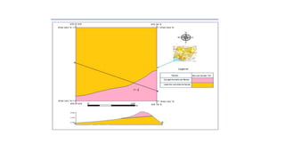
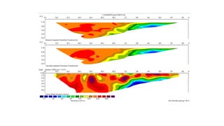
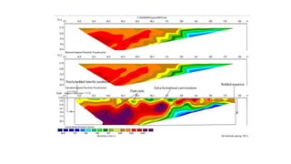
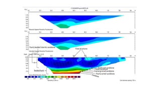
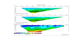
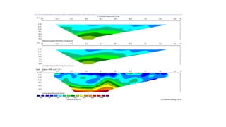
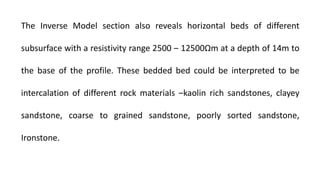
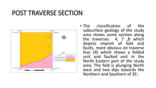
52. The Inverse Resistivity Model Section of Profile 1 (fig ) depicts a high lateral variation in
resistivity ranging from about 400Ωm to 5000Ωm to a depth of 23m suggesting the
presence of lateritic materials in top layer‒on the southern part of the profile section.
Within the poorly bedded lateritic sandstone high resistivity, are patches of Ironstone cast
deposition with resistivity values >3300Ωm. Towards the base of the Northern part of the
profile sections are layers of bedded sequences. These layers could be interpreted to be
intercalation of different rock materials with varying resistivity values [80Ωm ‒ 12000Ωm]
‒ consisting of clay, kaolin, clayey sandstone and medium to coarse grained sandstone.

54. The Inverse Resistivity Model Section of Profile 2 (fig ) reveals a general
disorderly range of resistivity values, 450Ωm ‒ 5500Ωm from the
surface to a depth of about 22m in thickness. Indicating a poorly
bedded lateritic sandstone regolith (a region of unconsolidated rock and
dust) towards the Southern part of the model section. The model
section shows zone of sedimentary structures, within the poorly
bedded lateritic sandstone known as flute casts.

55. The very high resistivity >5000Ωm geological formation observed between
98 ‒ 110m on the profile line at a depth of about 7‒11m shows a patch of
extra formational cast of ironstone deposit. This model sections also reveals
layers of the bedded sequence having a very low dip of about less than 5◦
towards the base of the Northern part of the profile. With a resistivity
values ranging from about 80Ωm to 1400Ωm indicating the presence of
clay, kaolin and clayey sandstone.

57. The Inverse Resistivity Model Section of Profile 3 (fig) section generally displays
wide range of resistivity values from 300 to about 7000Ωm to a depth to the
base beneath the profile, which signifies a heterogeneous lateritic top soil
formation ‒ as seen on the first part of the profile section. The resistivity model
section further unfolds within the lateritic material formation, sole structures
seen on the bottom of the top layer bed between 50 ‒ 90m along the profile.

58. Also seen within the poorly bedded lateritic sandstone are patches of ironstone
deposits at a resistivity values (˃6000Ωm) geological formation at the base
observed between 50m and 93m beneath the profile. The model section further
reveals layers of different surface materials bedded with resistivity values from
about 70 to 1600Ωm at depth about 12m to the base of the profile. These layers
could be interpreted to be intercalation of different rock materials ‒ including
clay, kaolin, clayey sandstone and a pocket of kaolin cast within the bedded
sequence.

60. The Inverse Resistivity Model Section of Profile 4 (fig) portrays high heterogeneities with
large resistivity variation (>200Ωm) from the surface up to a depth of about 20m, beneath
the profile reflecting a poorly bedded lateritic sandstone. Within the resistivity zone are
sedimentary structures ‒ flute casts and a pocket of kaolin cast at a resistivity of about
700Ωm. The very higher resistivity (>2300Ωm) geological formation labelled folded beds
shows an upward movement towards the top surface. The folded structures must have been
formed by an unequal loading of the overburden bed that led to the expansion of the
underneath beds into the overlying beds thus forming folds ‒ hence localized.

61. . During the folding process, the beds stretches beyond elastic limit resulting
in a deformational structure ‒ fault. The localized folded beds corroborates
with the observation made by Salafu and Ujuanbi (2015) “On the occurrence
of deformational structures in some part of Esan Land”. The deformed
bedded sequence as seen from the profile model section from the surface up
to a depth of about 18m, with resistivity values ranging from 60Ωm to about
400Ωm beneath the profile on the Northern part of the profile section.

63. The Inverse Resistivity Model Section of Profile 5 (figure) shows
varying range of resistivity from 400Ωm ‒ 2000Ωm along the entire
profile length to a depth of about 10m from the surface indicating a
poorly bedded lateritic sandstone. Within the poorly bedded
lateritic sandstone are zones of sedimentary structures between
36m ‒ 60m and 82m ‒ 88m. These zones were interpreted as flutes
structures.

64. The resistivity model also bring to light a thin resistivity high
values >200Ωm formation between 22 ‒ 44m, which extend from
a depth 10m to the base of the model section. The bedded bed
have very low dip of about less than 5◦ revealing a sequence of
bedded Ironstone, poorly sorted sandstone, coarse to medium
grained sandstone, clayey sandstone, and kaolin rich sandstone.

66. The Inverse Resistivity Model of Profile 6 (figure ) section shows varying high resistivity
values (900Ωm ‒ 8000Ωm) along the entire profile length and up to a depth of about
15m beneath the profile. This could be attributed to weathering effect and lateritic
materials in the top layer. The resistivity model section also reveals a uniform bedded
sequence underlying the poorly lateritic sandstone zone with a resistivity value
˃3000Ωm. Extending from a depth of 15m to the base of the model sections. The
layered beds reveals coarse grained sandstone, poorly sorted sandstone, Ironstone
ferruginized sandstone.

68. The profile section (fig) shows varying resistivity range 400Ωm ‒ 3000Ωm
from the surface up to a depth of 12m beneath the profile. Indicating the
presence of lateritic materials in the top layer. There are two protruded high
resistivity (˃3000Ωm) geological formation ‒ folded beds observed between
24m to 90m beneath the profile. The folded beds formed probably as a
result of an unequal loading of the overburden beds leading to the
expansion of the underneath beds into the overlying beds thus forming fold.

70. The Inverse Resistivity Model Section of Profile 8 (figure) shows varying
resistivity top layer values from about 200Ω to 1200Ωm to a depth of about
11m indicating a weathered top layer ‒ poorly bedded lateritic sandstone.
There is a protruded high resistivity ˃1400Ωm deformational structure (fold)
observed between 50 ‒ 85m on the other half of the section. The folded beds
is similar to profile 7 formed as a result of unequal loading of the overburden
beds ‒ a case of differential in settlement.

72. The Inverse Resistivity Model section of Profile 9 (figure) produces two different
geological layered rock, which are clearly defined by their resistivity layers at the
various depths. The Inverse Resistivity Model Section reveals wide range of
resistivity values 200 ‒ 2300Ωm to a depth of about 14m from the surface. This
layer can be interpreted as poorly bedded lateritic sandstone indicating a highly
weathered top soil formation.

73. The Inverse Model section also reveals horizontal beds of different
subsurface with a resistivity range 2500 ‒ 12500Ωm at a depth of 14m to
the base of the profile. These bedded bed could be interpreted to be
intercalation of different rock materials ‒kaolin rich sandstones, clayey
sandstone, coarse to grained sandstone, poorly sorted sandstone,
Ironstone.

74. SUBSURFACE LITHO-STRUCTURAL CLASSIFICATION
OF THE STUDY AREA
• The geoelectric lithologs for
traverse model sections 1, 2, 3, 4,
and 7 layered stratas have been
affected by structures within, in
this case the layers are not longer
horizontal. Therefore no equal
resistivity values within a
geological strata. The layers have
been distorted and overtured by
the geological structures within
them, with a non-homogenous
resistivity value.
• The geoelectric lithologs for
traverse model sections 5, 6, 8 and
9 (Figure) shows a relatively high
level of conformity, yet to be
distorted with the insitu deposit
still in place. As seen from the
lithologs section, the layers of
sediment extends laterally in all
direction

75. SUBSURFACE LITHO-STRUCTURAL CLASSIFICATION
OF THE STUDY AREA

76. SUBSURFACE LITHO-STRUCTURAL CLASSIFICATION
OF THE STUDY AREA

77. POST TRAVERSE SECTION
• The classification of the
subsurface geology of the study
area shows some section along
the traverses 4, 7 ,8 which
depicts imprint of fold and
faults, more obvious on traverse
four (4) which shows a folded
unit and faulted unit in the
North Eastern part of the study
area. The fold is plunging North
west and two dips towards the
Northern and Southern of 35◦.

78. CONCLUSION
The 2D ERT resistivity technique produced substantial 2D inverse model section
with high quality in terms of structural resolution, as against the poor subsurface
resolution often associated with conventional electrical methods. It gave a
clearer view and delineation of various lithological units of the subsurface in the
area, and clear image of sedimentary structures (sole cast extra formational cast
and flute cast) and deformational structures (fault and fold).

79. The Electrical Resistivity Tomography result when correlated with
borehole data from Ekpoma shows that 80Ωm - 150Ωm gives clay
signature, 160Ωm ‒ 400Ωm gives kaolin signature, 400Ωm ‒ 1039Ωm
represents clayey sandstone, 1100Ωm ‒ 3999Ωm signifies medium to
coarse grained sandstone, and 4000 ‒ 44000Ωm represent Ironstone ‒
ferruginized sandstone.

80. RECOMMENDATION
A 2-Dimensional Resistivity Imaging has been carried out within the study area to
classify the subsurface earth, the following recommendations are given.
i. Henceforth, future researchers should employ Electrical Resistivity Tomography
in classifying the subsurface, in order to pick out Sedimentary Structures.
ii. Based on the research work, Borehole Drilling should be carried out on some
traverses (2 and 4) for some groundtruthing.

81. CONTRIBUTION TO KNOWLEDGE
1. The research work was able to provide a more accurate model of the
subsurface within the study area, which before now was not available.
2. The study work was able to establish the trend of resistivity variation
both vertically and laterally within the study area.
3. The research work will serve as a case study for future researchers and
developers in erecting structures within the sport complex vicinity.

82. Aizebeokhai, A. P. (2010). 2D and 3D Geoelectrical resistivity imaging: Theory and field design. Scientific
Research and Essays, 5(23), 3592-3605.
Alile, O.M., & Ehigiator, M.O. (2011). Determination of the aquifer layer by the application of electrical method
of exploration at Ubiaja in Edo Central of Nigeria. Scientific Research and Essays Vol. 6(2), pp. 493-498.
Aminu, M.B. (2015). Electrical Resistivity Imaging of a Thin Clayey Aquitard Developed on Basement Rocks in
Parts of Adekunle Ajasin University Campus, Akungba-Akoko, South-Western Nigeria. Environmental
Research, Engineering
Ayolabi, E. A., Folorunso, A. F., Eleyinmi, A. F., & Anuyah, E. O. (2009c). Applications of 1D and 2D
electrical resistivity methods to map aquifers in a complex geologic terrain of Foursquare Camp,
Ajebo, southwestern Nigeria. Pacific Journal of Science and Technology, USA, 10(2), 657-666.
Ayolabi, E. A., Atakpo, E. A., Adeoti, L., Otobor, E. C., & Arerin, T. (2009b). Groundwater quality assessment
using predrilling electrical measurements. Journal of Environmental Hydrology, 17, 1-12.
Ayolabi, E. A., Folorunso, A.F., and Idem, S. S. (2012). Application of Electrical Resistivity Tomography in
Mapping Subsurface Hydrocarbon Contamination. Canadian Center of Science and Education. Earth Science
Research, vol.2, no 1, pp. 93-103.

83. Ayolabi, E. A., Folorunso, A.F. and Jegede, O.E. (2013). An Application of 2D Electrical Resistivity Tomography
in Geotechnical Investigation of Foundation Defects: A Case Study. Journal of Geology and Mining Research,
vol. 3, no. 12, pp. 142-151.
Bayemu, O.O., Oloruntola, M.O., Mosuro, G.O., (2012). Application of electrical resistivity imaging (ERI) in
delineating anon-conformity around Ijesha-Ijebu, Southwestern Nigeria. Journal of Petroleum and Gas
Exploration Research, 010-016.
Cahyna, F., Mazac, O., & Vendhova, D. (1990). Determination of the extent of cyanide contamination by
surface geo-electrical methods. SEG- Geotechnical and environmental Geophysics, Tulsa, 2, 97-99.
Egwuonwu, G.N., S.O. Ibe, and I.B. Osazuwa. (2011). Geophysical Assessment of foundation Depths around a
Leaning Superstructure in Zaria Area, Northwestern Nigeria using Electrical Resistivity Tomography. Pacific
Journal of Science and Technology. 12(1): 472-486. http://www.akamaiuniversity.us/PJST.htm
Edwards, L. S. (1997). A modified pseudosection for resistivity and induced polarization (IP)
Folorunso, A.F., Ayolabi, E.A; Ariyo, S.O., Oyebanjo, I.O. (2012). Fault Presence under a failing Building Complex
mapped by electrical resistivity tomography. Mineral Wealth, Greece. 47-55.

84. Giao, P. H., Chung, S. G., Kim, D. Y., & Tanaka, H. (2003). Electrical imaging and laboratory resistivity testing for
geotechnical investigation of Pusan clay deposits. Journal of Applied Geophysics, 52, 157-175.
Gibson, P. J. and George, M. D. (2003). Environmental Application of Geophysical Surveying Techniques.
Hauppauge: Nova Science Publishers.
Geotomo Software, 2010. Geoelectrical Imaging 2D & 3D Geotomo Software (RES2DINV ver. 3.59) manual.
Minden Heights, 11700 Gelugor (Penang):
Griffiths, D.H. and Barker, R.D., (1993). Two-dimensional resistivity imaging and modeling in areas of complex
geology. J. Appl. Geophys., 1993, 29, 211-226.
Kearey, P. and Brooks, M. (1991). An Introduction to Geophysical Exploration. London: Blackwell Scientific
Publication.
Kearey, P., Brooks, M., and Hill, I., (2002). An introduction to geophysical exploration (Third Edition). Blackwell
Publishing, Malden, U.S.A. pp. 66-67
Khalil, M. H. (2009). Hydrogeophysical assessment of wadi el-sheikh aquifer, saint katherine, south Sinai, Egypt.
Journal of Environmental and Engineering Geophysics, JEEG, 14(2), 77-86.
http://dx.doi.org/10.2113/JEEG14.2.77

85. Loke, M.H. (2002). Electrical imaging surveys for environmental and engineering studies, a practical guide to 2-D and
3-D surveys.
Loke, M. H. and Barker, R.D, (1996). Rapid least-squares inversion of apparent resistivity pseudosection by a quasi-
Newton method. Geophysical Prospecting, vol. 44, pp. 131-152
Loke, M. H., (2004). Rapid 2-D resistivity and IP inversion using the least-square method; Manual for Res2dinv,
version 3.54.53p
Lowrie, W. (1997). Fundamentals of Geophysics. Cambridge University press. 345p.
Mondal N.C., Rao V.A., Singh V.S. and Sarwade D.V. (2008). Delineation of concealed lineaments using electrical
resistivity imaging in granitic terrain. Current Science. 94(3): 277-283.
Mwenifumbo, C. J. (1997). Electrical methods for Ore body delineation, Proceeding of Exploration 97: Fourth
Decennial International Conference on Mineral Exploration, A.G Gubbins (Ed.). pp. 667-676.
Oyeyemi, K.D., and Olofinnade, O.M. (2016). Geoelectrical – Geotechnical studies for Near Surface characterization,
Case History: Lagos, SW Nigeria. Electronic Journal of Geotechnical Engineering., 3735-3750.
Osazuwa, I.B. and Abdullahi N.K., (2008). Electrical resistivity and Induced Polarization Investigation at an open
Solid Waste Dumpsite. Case Study: Kaduna. Journal of Environmental Hydrology, vol. 16, no 29, pp 1-11.

86. Osazuwa, I.B. and Chii, E.C. (2009). A two-dimensional electrical resistivity imaging of an earth dam, Zaria,
Nigeria. Journal of Environmental Hydrology, vol. 17.
Parasins, D. S. (1962). Principles of applied geophysics. London: Methuen & Co Ltd., pp108.
Pellerin, L. (2002). Applications of electrical and electromagnetic methods for environmental and geotechnical
Investigations. Surveys in Geophysics, vol. 23, pp. 101-132
Ramazi, H., Nejad, M. R. H., & Aenollah, A. F. (2009). Application of intergrated methods in Khenadarreh
(Arak, Iran) Graphite deposit exploration. Journal Geological Society of India, 74, 260-266.
http://dx.doi.org/10.1007/s12594-009-0126-5
Salufu, S.O., & Ujuanbi, O. (2015). OCCURRENCE OF DEFORMATIONAL STRUCTURES IN THE PALEOCENE-EOCENE
SEDIMENTS IN ESAN LAND, EDO STATE NIGERIA. NIGERIAN ANNALS OF NATURAL SCIENCES, VOLUME 15 (1)
2015 (pp 085 –093)
Venkateswarlu, G., Jayasankar, G. and Saradhi, B. V. (2014). Impact assessment of land use change on ground
water quality using remote sensing and GIS for zone V under municipal corporation hyderbad. IOSR Journal
of Mechanical and Civil Enginnering, vol. 11, no. 1, pp. 36-42.
Zohdy AAR. The auxiliary point method of electrical sounding interpretation, and its relationship to the Dar
zarrouk parameters. Geophys. 1965; 3(4):644-650.