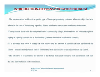
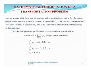
The document discusses the transportation problem and how to solve it. The transportation problem aims to minimize the cost of transporting goods from multiple sources to multiple destinations, given supply and demand constraints. It describes the mathematical formulation and defines key terms like feasible and basic feasible solutions. It also outlines several methods to obtain the initial basic feasible solution, including the Northwest Corner Rule, Least Cost Method, and Vogel's Approximation Method. Finally, it discusses the Modi Method for obtaining the optimal basic solution through iterative testing of cell evaluations.

1. TRANSPORTATION
PROBLEM
PROBLEM

2. Dr. K . BHARATHI
Assistant Professor of Mathematics,
Sri Chandrasekharendra Saraswathi Viswa Mahavidyalaya,
Sri Chandrasekharendra Saraswathi Viswa Mahavidyalaya,
Kanchipuram.
kbharathi@kanchiuniv.ac.in

3. CONTENT
 OBJECTIVES OF TRANSPORTATION PROBLEM
 INTRODUCTION TO TRANSPORTATION PROBLEM
 MATHEMATICAL FORMULATION OF A TRANSPORTATION PROBLEM
 INITIAL BASIC FEASIBLE SOLUTION
 OPTIMAL BASIC SOLUTION - MODI METHOD - MODIFIED
DISTRIBUTION METHOD
 ASSIGNMENT QUESTIONS
 MCQ QUESTIONS WITH ANSWER
K.BHARATHI, Assistant Professor of Mathematics,
SCSVMV 3

4. OBJECTIVES OF TRANSPORTATION PROBLEM
• Transportation problem works in a way of minimizing the cost function.
• The cost function is the amount of money spent to the logistics provider for
transporting the commodities from production or supplier place to the
demand place.
4
K.BHARATHI, Assistant Professor of Mathematics,
SCSVMV
• It includes the distance between the two locations, the path followed, mode
of transport, the number of units that are transported, the speed of
transport, etc.
• To transport the commodities with minimum transportation cost without
any compromise in supply and demand.

5. INTRODUCTION TO TRANSPORTATION PROBLEM
• The transportation problem is a special type of linear programming problem, where the objective is to
minimize the cost of distributing a product from a number of sources to a number of destinations.
•Transportation deals with the transportation of a commodity (single product) from ‘m’ sources (origin or
supply or capacity centres) to ‘n’ destinations (sinks or demand or requirement centres).
supply or capacity centres) to ‘n’ destinations (sinks or demand or requirement centres).
• It is assumed that, level of supply of each source and the amount of demand at each destination are
known . The unit transportation cost of commodity from each source to each destination are known.
• The objective is to determine the amount to be shifted from each source to each destination such that
the total transportation cost is minimum.
5
K.BHARATHI, Assistant Professor of Mathematics,
SCSVMV

6. MATHEMATICAL FORMULATION OF A
TRANSPORTATION PROBLEM
Let us assume that there are m sources and n destinations. Let ai be the supply
(capacity) at source i, bj be the demand at destination j, cij be the unit transportation
cost from source i to destination j and xij be the number of units shifted from source i
to destination j.
Then the transportation problem can be expressed mathematically as,
Minimize Z =
m n
c x
  subject to the constraints,
Minimize Z =
1 1
ij ij
i j
c x
 
  subject to the constraints,
1
1
, 1, 2,
, 1, 2,
0, ,
n
ij i
j
m
ij j
i
ij
x a i m
x b j n
x i j


 
 
 




6
K.BHARATHI, Assistant Professor of Mathematics,
SCSVMV

7. REMARK
 The two sets of constraints will be consistent, if
1 1
m n
i j
i j
a b
 

  , (ie.,Total Supply = Total
Demand) which is the necessary and sufficient for a transportation problem to have a feasible
solution.
 Problem satisfying this condition are called as balanced transportation problem. If not, then
the transportation problem is called an unbalanced one.
 If the given transportation problem is an unbalanced problem one has to balance the
transportation problem first.
7
K.BHARATHI, Assistant Professor of Mathematics,
SCSVMV
 When the total supply is greater than the total demand, a dummy is destination is included in
the matrix with zero cost elements and the excess supply is entered as a constraint for the
dummy destination.
 When the total demand is greater than the total supply, a dummy source is included in the
matrix with zero cost elements and the excess demand is entered as a constraint for the
dummy source.

8. STANDARD TRANSPORTATION TABLE
Transportation problem is explicitly represented by the following transportation table,
Destination
Supply
D1 D2 D3 … Dj … Dn
Source
S1 c11 c12 c13 … c1j … c1n a1
S2 c21 c22 c23 … c2j … c2n a2
S3 c31 c32 c33 … c3j … c3n a3
   …  … 
Si ci1 ci2 ci3 … cij … cin ai
K.BHARATHI, Assistant Professor of Mathematics,
SCSVMV 8
c c c c c
   …  … 
Sm cm1 cm2 cm3 … cmj … cmn am
Demand b1 b2 b3 bj bn i j
a b
 

The mn squares are called cells. The various a’s and b’s are called the constraints (rim
conditions)

9. BASIC DEFINITIONS
• Feasible Solution: A set of non-negative values xij, i = 1, 2 … m; j = 1, 2 …n that satisfies the
constraints (rim conditions) is called a feasible solution.
• Basic Feasible Solution: A feasible solution to a (m x n) transportation problem that contains no more
that m + n – 1 non-negative independent allocations is called a basic feasible solution(BFS) to the
transportation problem.
• Non-Degenerate Basic Feasible Solution: A basic feasible solution to a (m x n) transportation
problem is said to be a non-degenerate basic feasible solution if it contains exactly m + n – 1 non-
K.BHARATHI, Assistant Professor of Mathematics,
SCSVMV 9
problem is said to be a non-degenerate basic feasible solution if it contains exactly m + n – 1 non-
negative allocations in independent positions.
• Degenerate Basic Feasible Solution: A basic feasible solution that contains less than m + n – 1 non-
negative allocations is said to be a degenerate basic feasible solution.
• Optimal Solution: A feasible solution (not necessarily basic) is said to be an optimal solution if it
minimises the total transportation cost.
• The number of basic variables in an m x n balanced transportation problem is at the most m + n – 1.

10. TYPES OF TRANSPORTATIONPROBLEM
• Balanced Transportation Problem: where the total
supply equals to the total demand
• Unbalanced Transportation Problem: where the
total supply is not equal to the total demand
10
K.BHARATHI, Assistant Professor of Mathematics,
SCSVMV

11. PHASES OF SOLUTION OF TRANSPORTATION PROBLEM
• Phase I- obtains the initial basic feasible solution
• Phase II-obtains the optimal basic solution
• Phase II-obtains the optimal basic solution
Optimality condition: m+n-1 no of allocation
Where m= number of rows and n=
number of columns
11
K.BHARATHI, Assistant Professor of Mathematics,
SCSVMV

12. INITIAL BASIC FEASIBLE SOLUTION
The following methods are to find the initial basic feasible
solution for the transportation problems.
• North West Corner Rule (NWCR)
• North West Corner Rule (NWCR)
• Least Cost Method
• Vogle’sApproximation Method(VAM)
12
K.BHARATHI, Assistant Professor of Mathematics,
SCSVMV

13. METHOD 1: NORTH-WEST CORNER RULE
Step 1: The first assignment is made in the cell occupying the upper left-hand (north-west) corner of
the transportation table. The maximum possible amount is allocated there. That is, x11 = min {a1, b1}.
i. If min {a1, b1} = a1, then put x11= a1, decrease b1 by a1 and move vertically to the
2nd
row (to the cell (2, 1)) and cross out the first column.
ii. If min {a , b } = b , then put x = b , decrease a by b and move horizontally
13
K.BHARATHI, Assistant Professor of Mathematics,
SCSVMV
ii. If min {a1, b1} = b1, then put x11= b1, decrease a1 by b1 and move horizontally
right (to the cell (1, 2)) and cross out the first column.
iii. If min {a1, b1} = a1 = b1, then put x11= a1 = b1 and move diagonally to the cell (2,
2) cross out the first row and the first column.
Step 2: Repeat the procedure until all the rim requirements are satisfied.

14. METHOD 2: LEAST COST METHOD (OR) MATRIX MINIMA METHOD (OR) LOWEST
COST ENTRY METHOD
Step 1: Identify the cell with smallest cost and allocate xij = min {ai, bj}.
i. If min {ai, bj} = ai, then put x11= ai, cross out the ith
row and decrease bj by ai and
go to step (2).
ii. If min {ai, bj} = bj, then put x11= bj, cross out the jth
column and decrease ai by bj,
K.BHARATHI, Assistant Professor of Mathematics,
SCSVMV 14
and go to step (2).
iii. If min {ai, bj} = ai = bj, then put x11 = ai = bj, cross out either ith row or jth column
but not both and go to step (2).
Step 2: Repeat step (1) for the resulting reduced transportation table until all the rim requirements
are satisfied.

15. METHOD 3: VOGEL’S APPROXIMATION METHOD (OR) UNIT COST PENALTY
METHOD
Step1: Find the difference (penalty) between the smallest and next smallest costs in each row
(column) and write them in brackets against the corresponding row (column).
Step 2: Identify the row (or) column with largest penalty. If a tie occurs break the tie arbitrarily.
Choose the cell with smallest cost in that selected row or column and allocate as much as possible to
K.BHARATHI, Assistant Professor of Mathematics,
SCSVMV 15
Choose the cell with smallest cost in that selected row or column and allocate as much as possible to
this cell and cross out the satisfied row or column and go to step (3).
Step 3: Again compute the column and row penalties for the reduced transportation table and then
go to step (2). Repeat the procedure until all the rim requirements are satisfied.

16. PROBLEM 1: Obtain initial feasible solution for the following Transportation
table using (i) North West Corner rule. (ii) Least Cost Method. (iii) VAM
Method.
K.BHARATHI, Assistant Professor of Mathematics,
SCSVMV 16

17. K.BHARATHI, Assistant Professor of Mathematics,
SCSVMV 17
The given problem is balanced 𝑖
𝑚
𝑖=1 𝑗
𝑛
𝑗 =1 ,
ie.,Total Supply = Total Demand

18. To find the IBFS using (i) North West Corner rule:
The number of allocations = 6 = 4+3-1 = m+n-1, is a non-degenerate solution.
The IBFS is = (2*5)+(3*2)+(3*6)+(4*3)+(7*4)+(2*14) = 153.
K.BHARATHI, Assistant Professor of Mathematics,
SCSVMV 18

19. To find the IBFS using (ii) Least Cost Method
The number of allocations = 6 = 4+3-1 = m+n-1, is a non-degenerate solution.
The IBFS is = (7*2)+(4*3)+(1*8)+(4*7)+(1*7)+(2*7) = 83.
K.BHARATHI, Assistant Professor of Mathematics,
SCSVMV 19

20. To find the IBFS using (iii) VAM
The number of allocations = 6 = 4+3-1 = m+n-1, is a non-degenerate solution.
The IBFS is = (2*5)+(3*2)+(1*6)+(4*7)+(1*2)+(2*12) = 76.
K.BHARATHI, Assistant Professor of Mathematics,
SCSVMV 20

21. OPTIMAL BASIC SOLUTION - MODI METHOD -
MODIFIED DISTRIBUTION METHOD
Step 1: Find the initial basic feasible solution of the given problem by Northwest Corner
Rule (or) Least Cost Method (or) VAM.
Step 2: Check the number of occupied cells. If there are less than m + n – 1, there exists
K.BHARATHI, Assistant Professor of Mathematics,
SCSVMV 21
Step 2: Check the number of occupied cells. If there are less than m + n – 1, there exists
degeneracy and we introduce a very small positive assignment of in suitable independent
positions, so that the number of occupied cells is exactly equal to m + n – 1.
Step 3: Find the set values ui, vj (i = 1, 2, …m ; j = 1, 2, …n) from the relation cij = ui + vj for
each occupied cell (i, j), by starting initially with ui = 0 or vj = 0 preferably for which the
corresponding row or column has maximum number of individual allocations.

22. Step 4: Find ui + vj for each unoccupied cell (i, j) and enter at the upper right corner of the
corresponding cell (i, j).
Step 5: Find the cell evaluations dij = cij – (ui + vj) for each unoccupied cell (i, j) and enter
at the upper left corner of the corresponding cell (i, j).
Step 6: Examine the cell evaluations dij for all unoccupied cells (i, j) and conclude that,
K.BHARATHI, Assistant Professor of Mathematics,
SCSVMV 22
Step 6: Examine the cell evaluations dij for all unoccupied cells (i, j) and conclude that,
•If all dij> 0, then the solution under the test is optimal and unique.
•If all dij> 0, with at least one dij = 0, then the solution under the test is optimal and an
alternative optimal solution exists.
•If at least one dij< 0, then the solution is not optimal. Go to the next step.

23. Step 7: Form a new BFS by giving maximum allocation to the cell for which dij is most
negative by making an occupied cell empty. For that draw a closed path consisting of
horizontal and vertical lines beginning and ending at the cell for which dij is most negative
and having its other corners at some allocated cells. Along this closed loop indicate +θ
and –θ alternatively at the corners. Choose minimum of the allocations from the cells
K.BHARATHI, Assistant Professor of Mathematics,
SCSVMV 23
and –θ alternatively at the corners. Choose minimum of the allocations from the cells
having –θ. Add this minimum allocation to the cells with +θ and subtract this minimum
allocation from the allocation to the cells with –θ.
Step 8: Repeat steps (2) to (6) to test the optimality of this new basic feasible solution.
Step 9: Continue the above procedure till an optimum solution is attained.

24. PROBLEM 1: Solve the Transportation table.
Source Destination Supply
A B C
1 2 2 3 10
K.BHARATHI, Assistant Professor of Mathematics,
SCSVMV 24
2 4 1 2 15
3 1 3 1 40
Demand 20 15 30

25. K.BHARATHI, Assistant Professor of Mathematics,
SCSVMV 25
The given problem is balanced 𝑖
𝑚
𝑖=1 𝑗
𝑛
𝑗 =1 ,
ie.,Total Supply = Total Demand

26. To find the IBFS using VAM
The number of allocations = 5 = 3+3-1 = m+n-1, is a non-degenerate solution.
The IBFS is = (2*10)+(1*5)+(2*10)+(1*20)+(1*20) = 85.
K.BHARATHI, Assistant Professor of Mathematics,
SCSVMV 26

27. To find the optimal solution using MODI Method:
 Find the set values ui, vj (i = 1, 2, …m ; j = 1, 2, …n) from the relation cij = ui + vj for each occupied cell (i, j), by starting
initially with ui = 0 or vj = 0 preferably for which the corresponding row or column has maximum number of individual
allocations.
 Find ui + vj for each unoccupied cell (i, j) and enter at the upper right corner of the corresponding cell (i, j).
 Find the cell evaluations dij = cij – (ui + vj) for each unoccupied cell (i, j) and enter at the upper left corner of the
corresponding cell (i, j).
K.BHARATHI, Assistant Professor of Mathematics,
SCSVMV 27

28. Form a new BFS by giving maximum allocation to the cell for which dij is most negative by
making an occupied cell empty. For that draw a closed path consisting of horizontal and
vertical lines beginning and ending at the cell for which dij is most negative and having its
other corners at some allocated cells. Along this closed loop indicate +θ and –θ alternatively at
the corners. Choose minimum of the allocations from the cells having –θ. Add this minimum
allocation to the cells with +θ and subtract this minimum allocation from the allocation to the
cells with –θ.
K.BHARATHI, Assistant Professor of Mathematics,
SCSVMV 28

29. K.BHARATHI, Assistant Professor of Mathematics,
SCSVMV 29
Since all dij > 0 the above allocation is optimal unique solution.
The Optimal solution = (2*10)+(1*15)+(2*0)+(1*30)+(1*10) = 75.

30. ASSIGNMENT QUESTIONS
1. Obtain initial feasible solution for the following Transportation table using (i)
North West Corner rule. (ii) Least Cost Method. (iii) VAM Method.
Source Destination Supply
A B C
1 7 3 4 2
2 2 1 3 3
3 3 4 6 3
Demand
4 1 3
K.BHARATHI, Assistant Professor of Mathematics,
SCSVMV 30
2. Solve the Transportation table.
Source
Destination
Supply
A B C D
1 5 4 2 6 20
2 8 3 5 7 30
3 5 9 4 6 50
Demand
10 40 20
30

31. MCQ QUESTIONS WITH ANSWER
(1) To find initial feasible solution of a transportation problem the method which starts
allocation from the lowest cost is called method.
(a) north west corner
(b) least cost
(c) south east corner
(d) Vogel’s approximation
(2) In a transportation problem, the method of penalties is called method.
(a) least cost
(b) south east corner
(c) Vogel’s approximation
(d) north west corner
(3) When the total of allocations of a transportation problem match with supply and demand
values, the solution is called solution.
(a) non-degenerate
(b) degenerate
(c) feasible
K.BHARATHI, Assistant Professor of Mathematics,
SCSVMV 31
(c) feasible
(d) infeasible
(4) When the allocations of a transportation problem satisfy the rim condition (m + n – 1) the
solution is called solution.
(a) degenerate
(b) infeasible
(c) unbounded
(d) non-degenerate
(5) When there is a degeneracy in the transportation problem, we add an imaginary allocation
called in the solution.
(a) dummy
(b) penalty
(c) epsilon
(d) regret

32. (6) If M + N – 1 = Number of allocations in transportation, it means .(Where ‘M’ is
number of rows and ‘N’ is number of columns)
(a) There is no degeneracy
(b) Problem is unbalanced
(c) Problem is degenerate
(d) Solution is optimal
(7) Which of the following considers difference between two least costs for each row and
column while finding initial basic feasible solution in transportation?
(a) North west corner rule
(b) Least cost method
(c) Vogel’s approximation method
(d) Row minima method
(8) The solution to a transportation problem with m-sources and n-destinations is feasible if the
numbers of allocations are ___________.
(a) m+n
(b) mn
(c) m-n
K.BHARATHI, Assistant Professor of Mathematics,
SCSVMV 32
(d) m+n-1
(9) When the total demand is equal to supply then the transportation problem is said to be
_________
(a) balanced
(b) unbalanced
(c) maximization
(d) minimization
(10) When the total demand is not equal to supply then it is said to be __________.
(a) balanced
(b) unbalanced
(c) maximization
(d) minimization

33. (11) The allocation cells in the transportation table will be called ____________ cell
(a) occupied
(b) unoccupied
(c) no
(d) finite
(12) In the transportation table, empty cells will be called ___________.
(a) occupied
(b) unoccupied
(c) basic
(d) non-basic
(13) In a transportation table, an ordered set of___________or more cells is said to form a loop
(a) 2
(b) 3
(c) 4
(d) 5
K.BHARATHI, Assistant Professor of Mathematics,
SCSVMV 33
(d) 5
(14) To resolve degeneracy at the initial solution, a very small quantity is allocated in
____________ cell
(a) occupied
(b) basic
(c) non-basic
(d) unoccupied
(15) For finding an optimum solution in transportation problem ____________ method is used.
(a) Modi
(b) Hungarian
(c) Graphical
(d) simplex

34. THANK YOU
K.BHARATHI, Assistant Professor of Mathematics,
SCSVMV 34
THANK YOU