Transportation and assignment problem

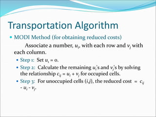
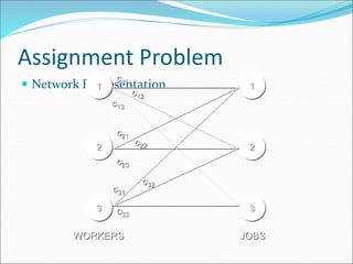
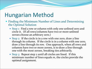
1. Operations Research (OR) 18UAMA31
II B.Sc Mathematics A & B
Mrs. G. Nagalakshmi
Mrs. K. Muthulakshmi
Miss. S. Swathi Sundari

2. Transportation Problem
 The transportation problem seeks to minimize
the total shipping costs of transporting goods
from m origins or sources (each with a supply
si) to n destinations (each with a demand dj),
when the unit shipping cost from source, i, to a
destination, j, is cij.
 The network representation for a
transportation problem with two sources and
three destinations is given on the next slide.

3. Transportation Problem
 LP Formulation
The linear programming formulation in terms of the
amounts shipped from the sources to the destinations, xij ,
can be written as:
Min cijxij (total transportation cost)
i j
s.t. xij < si for each source i (supply constraints)
j
xij = dj for each destination j (demand
constraints)
i
xij > 0 for all i and j (nonnegativity constraints)

4. Transportation Problem
 To solve the transportation problem by its special
purpose algorithm, it is required that the sum of
the supplies at the sources equal the sum of the
demands at the destinations. If the total supply is
greater than the total demand, a dummy
destination is added with demand equal to the
excess supply, and shipping costs from all sources
are zero. Similarly, if total supply is less than total
demand, a dummy source is added.
 When solving a transportation problem by its
special purpose algorithm, unacceptable shipping
routes are given a cost of +M (a large number).

5. Transportation Problem
 The transportation problem is solved in two phases:
 Phase I -- Obtaining an initial feasible solution
 Phase II -- Moving toward optimality
 In Phase I, the Minimum-Cost Procedure can be used to
establish an initial basic feasible solution without doing
numerous iterations of the simplex method.
 In Phase II, the Stepping Stone, by using the MODI
method for evaluating the reduced costs may be used to
move from the initial feasible solution to the optimal
one.

6. Initial Tableau
 There are many method for finding the initial tableau
for the transportation problem which are:
1. Northwest corner
2. Least cost
3. Vogle’s approximation method

7. Transportation Algorithm
 MODI Method (for obtaining reduced costs)
Associate a number, ui, with each row and vj with
each column.
 Step 1: Set u1 = 0.
 Step 2: Calculate the remaining ui's and vj's by solving
the relationship cij = ui + vj for occupied cells.
 Step 3: For unoccupied cells (i,j), the reduced cost = cij
- ui - vj.

8. Assignment Problem
 An assignment problem seeks to minimize the total cost
assignment of m workers to m jobs, given that the cost of
worker i performing job j is cij.
 It assumes all workers are assigned and each job is
performed.
 An assignment problem is a special case of a transportation
problem in which all supplies and all demands are equal to
1; hence assignment problems may be solved as linear
programs.
 The network representation of an assignment problem
with three workers and three jobs is shown on the next
slide.

9. Assignment Problem
 Network Representation
2
3
1
2
3
1
c11
c12
c13
c21
c22
c23
c31
c32
c33
WORKERS JOBS

10. Assignment Problem
 Linear Programming Formulation
Min cijxij
i j
s.t. xij = 1 for each worker i
j
xij = 1 for each job j
i
xij = 0 or 1 for all i and j.
 Note: A modification to the right-hand side of the first
constraint set can be made if a worker is permitted to work
more than 1 job.

11. Variations of Assignment Problem
 Total number of agents not equal to total number of
tasks
 Maximization objective function
 Unacceptable assignments

12. Hungarian Method
 The Hungarian method solves minimization
assignment problems with m workers and m jobs.
 Special considerations can include:
 number of workers does not equal the number of jobs --
add dummy workers or jobs with 0 assignment costs as
needed
 worker i cannot do job j -- assign cij = +M
 maximization objective -- create an opportunity loss
matrix subtracting all profits for each job from the
maximum profit for that job before beginning the
Hungarian method

13.  Step 1: For each row, subtract the minimum number in that
row from all numbers in that row.
 Step 2: For each column, subtract the minimum number in
that column from all numbers in that column.
 Step 3: Draw the minimum number of lines to cover all
zeroes. If this number = m, STOP -- an assignment can be
made.
 Step 4: Determine the minimum uncovered number (call it
d).
 Subtract d from uncovered numbers.
 Add d to numbers covered by two lines.
 Numbers covered by one line remain the same.
 Then, GO TO STEP 3.

14. Hungarian Method
 Finding the Minimum Number of Lines and Determining
the Optimal Solution
 Step 1: Find a row or column with only one unlined zero and
circle it. (If all rows/columns have two or more unlined
zeroes choose an arbitrary zero.)
 Step 2: If the circle is in a row with one zero, draw a line
through its column. If the circle is in a column with one zero,
draw a line through its row. One approach, when all rows and
columns have two or more zeroes, is to draw a line through
one with the most zeroes, breaking ties arbitrarily.
 Step 3: Repeat step 2 until all circles are lined. If this
minimum number of lines equals m, the circles provide the
optimal assignment.

15. Thank You