Downloaded 10 times

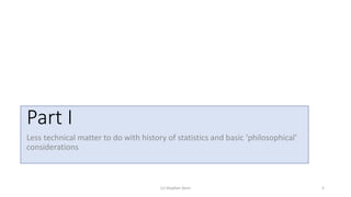


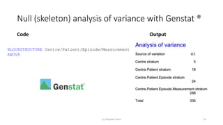
![Full (skeleton) analysis of variance with Genstat ®
Additional Code Output
(c) Stephen Senn 26
TREATMENTSTRUCTURE Design[]
ANOVA
(Here Design[] is a pointer with values corresponding
to each of the three designs.)](https://image.slidesharecdn.com/toinfinityandbeyondv2-201118220033/85/To-infinity-and-beyond-v2-26-320.jpg)


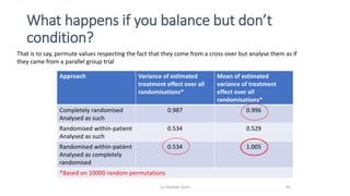


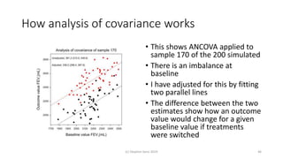

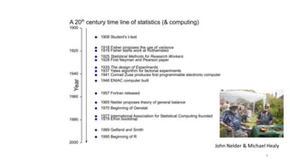
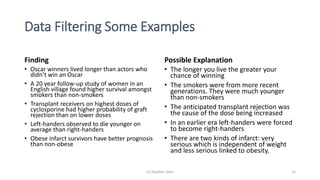
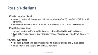
The document discusses the relationship between experiment design and data analysis, emphasizing that poorly designed studies can lead to misleading conclusions, regardless of the amount of data. It highlights the importance of careful experimental design while examining various statistical issues and challenges in clinical trials and observational studies. The author warns against over-reliance on big data claims, advocating for rigorous methodologies to ensure valid inferences.


![[DSC Europe 25] Bojan Djuricic - Predictive Design Process.pdf](https://cdn.slidesharecdn.com/ss_thumbnails/5awdrbedqdek3gqu2ezy-4-the-predictive-design-bojan-djuricic-260120105856-6c399e9b-thumbnail.jpg?width=640&height=640&fit=bounds)


![[DSC Europe 25] Elena Menshikova - AI-Powered Operational Excellence: Revolut...](https://cdn.slidesharecdn.com/ss_thumbnails/es6nholbqy3zaao2c2yd-2-elena-menshikova-data-ai-in-decision-making-260115093812-4fba8b38-thumbnail.jpg?width=640&height=640&fit=bounds)

![[DSC Europe 25] Nikola Vasiljevic - Player segmentation by combat playstyles ...](https://cdn.slidesharecdn.com/ss_thumbnails/mnvbf0yvrwaqsipzrrv3-2-nikola-vasiljevic-player-segmentation-by-playstyles-in-action-shooter-games-260114111931-b4d766cd-thumbnail.jpg?width=640&height=640&fit=bounds)
![[DSC Europe 25] Dragan Jerosimovic - The Anatomy of a Narrative Simulation.pdf](https://cdn.slidesharecdn.com/ss_thumbnails/vzputuprdqr6zwbrwdcw-1-dragan-jerosimovic-the-anatomy-of-a-narrative-simulation-260114111931-9d04fba2-thumbnail.jpg?width=640&height=640&fit=bounds)


![[DSC Europe 25] Ivan Lukovic & Marija Djukic - From Data to Value: Why Maturi...](https://cdn.slidesharecdn.com/ss_thumbnails/ahrfps8xr6knowwhacxh-1-ivan-marija-dsc-2025-ld-v1-presentation-260115093812-be21adfc-thumbnail.jpg?width=640&height=640&fit=bounds)
![[DSC Europe 25] Slobodan Dolinic - Smart and Intelligent Green Region.pptx](https://cdn.slidesharecdn.com/ss_thumbnails/0bribinjsp6ghwtvsvor-2-sigre-slobodan-dolinic-260115093812-c9c10e90-thumbnail.jpg?width=640&height=640&fit=bounds)