Downloaded 18 times


![Some references
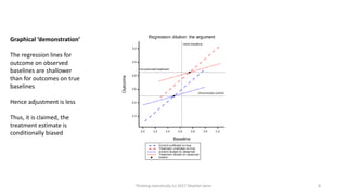
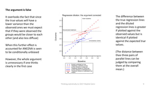
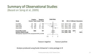
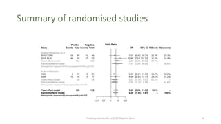
Thinking statistically (c) 2017 Stephen Senn 45
Senn, S. J. (1987). Correcting for regression in assessing the response to treatment in a selected population [letter].
Statistics in Medicine, 6(6), 727-728
Senn, S. J. (1998). Mathematics: governess or handmaiden? Journal of the Royal Statistical Society Series D-The
Statistician, 47(2), 251-259
Senn, S. J. (1994). Methods for assessing difference between groups in change when initial measurement is subject
to intra-individual variation [letter; comment] [see comments]. Statistics in Medicine, 13(21), 2280-2285
Senn, S. (2008). A note concerning a selection "Paradox" of Dawid's. American Statistician, 62(3), 206-210
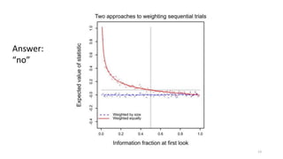
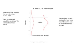
Senn, S. (2014). A note regarding meta-analysis of sequential trials with stopping for efficacy. Pharmaceutical
statistics, 13(6), 371-375
Senn, S. (2012). Misunderstanding publication bias: editors are not blameless after all. F1000Research, 1
Senn, S. (2013). Authors are also reviewers: problems in assigning cause for missing negative studies.
F1000Research. Retrieved from http://f1000research.com/articles/2-17/v1
stephen.senn@lih.lu](https://image.slidesharecdn.com/thinkingstatisticallyv3-170518185859/85/Thinking-statistically-v3-45-320.jpg)

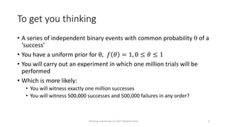
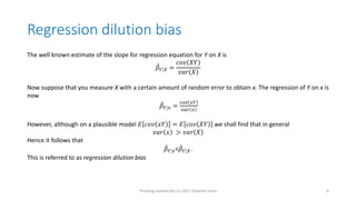
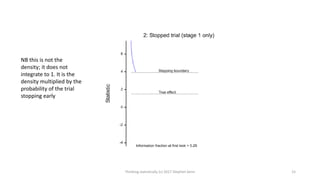
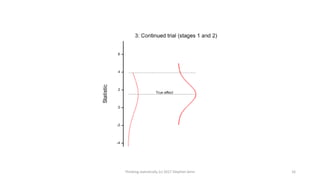
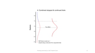
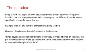
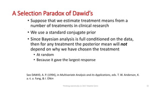
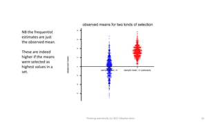
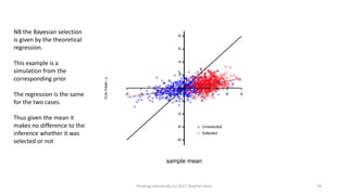
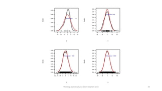
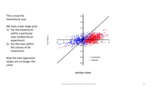
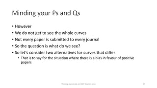
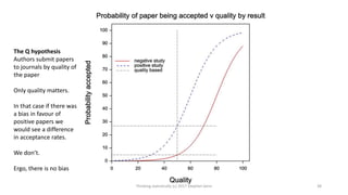
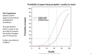
This document provides an overview of four statistical "paradoxes": 1) Covariate measurement error in randomized clinical trials, 2) Meta-analysis of sequential trials, 3) Dawid's selection paradox, and 4) Publication bias in the medical literature. For each paradox, brief explanations are given of the statistical issues involved and how they can be understood. Key points include that meta-analysis of sequential trials can account for early stopping by weighting trials by information amount, Dawid's selection paradox shows that Bayesian analysis is unaffected by selection of optimal outcomes, and publication bias may appear as a difference in acceptance rates between positive and negative results but could also be explained by differences in paper quality and targeting of journals. Graphs and heuristics