Downloaded 30 times


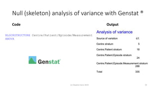
![Full (skeleton) analysis of variance with Genstat ®
Additional Code Output
(c) Stephen Senn 2019 20
TREATMENTSTRUCTURE Design[]
ANOVA
(Here Design[] is a pointer with values corresponding
to each of the three designs.)](https://image.slidesharecdn.com/understandingrandomisationv2-190804160006/85/Understanding-randomisation-20-320.jpg)
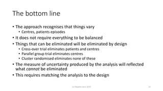
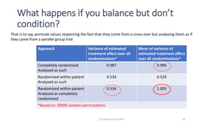

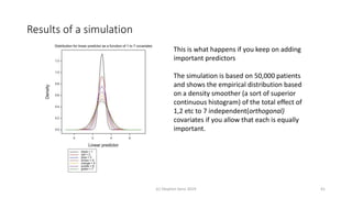


Randomisation balances both known and unknown factors that influence outcomes between treatment groups on average. Conditioning the analysis on available baseline covariates further reduces uncertainty by accounting for imbalances. While there are many potential covariates, their combined influence is bounded; randomisation thus remains important for accounting for unknown factors. Correct analysis requires matching the randomisation design to the analysis to make valid statistical inferences.