The paper discusses solutions to the economic dispatch problem in electric power systems using Ant Lion Optimization Algorithm (ALOA) and Bat Algorithm (BA) techniques. These methods aim to optimize electricity generation from various sources to meet demand while minimizing costs and carbon emissions. The algorithms were tested on a small and large-scale generator system, demonstrating their effectiveness in economic dispatch studies compared to other optimization methods.

1. International Journal of Electrical and Computer Engineering (IJECE)
Vol. 12, No. 3, June 2022, pp. 2228~2241
ISSN: 2088-8708, DOI: 10.11591/ijece.v12i3.pp2228-2241  2228
Journal homepage: http://ijece.iaescore.com
Economic dispatch by optimization techniques
Rana Ali Abttan1
, Adnan Hasan Tawafan2
, Samar Jaafar Ismael3
1
Computer Techniques Engineering Department, Baghdad College of Economic Sciences University, Baghdad, Iraq
2
Karbala Technical Institute, Al-Furat Al-Awsat Technical University, Baghdad, Iraq
3
Electromechanical Engineering Department, University of Technology, Baghdad, Iraq
Article Info ABSTRACT
Article history:
Received Apr 17, 2021
Revised Nov 7, 2021
Accepted Nov 30, 2021
The current paper offers the solution strategy for the economic dispatch
problem in electric power system implementing ant lion optimization
algorithm (ALOA) and bat algorithm (BA) techniques. In the power
network, the economic dispatch (ED) is a short-term calculation of the
optimum performance of several electricity generations or a plan of outputs
of all usable power generation units from the energy produced to fulfill the
necessary demand, although equivalent and unequal specifications need to
be achieved at minimal fuel and carbon pollution costs. In this paper, two
recent meta-heuristic approaches are introduced, the BA and ALOA. A
rigorous stochastically developmental computing strategy focused on the
action and intellect of ant lions is an ALOA. The ALOA imitates ant lions'
hunting process. The introduction of a numerical description of its biological
actions for the solution of ED in the power framework. These algorithms are
applied to two systems: a small scale three generator system and a large
scale six generator. Results show were compared on the metrics of
convergence rate, cost, and average run time that the ALOA and BA are
suitable for economic dispatch studies which is clear in the comparison set
with other algorithms. Both of these algorithms are tested on IEEE-30 bus
reliability test system.
Keywords:
Ant lion optimization
Bat algorithm optimization
Economic dispatch
IEEE-30
This is an open access article under the CC BY-SA license.
Corresponding Author:
Rana Ali Abttan
Computer Techniques Engineering Department, Baghdad College of Economic Sciences University
Baghdad, Iraq
Email: rana.ali.abttan@baghdadcollege.edu.iq
1. INTRODUCTION
In the economic system, economic dispatch has a fundamental role in assuring reliability and
security in the electric power system. The process of obtaining the optimal operation in the electrical power
systems is a difficult task that many have sought to find a solution to, due to the increase in the size of the
system and the number of variables and limitations of each issue as well as depends on the nature of the goal
to be reduced according to fixed conditions, so became the trend to use optimization inspired by nature. The
key purpose of the economic dispatch is to deploy the load economically and physically inside the units
concurrently. For e.g., variables influencing running costs, such as load distance generator, fuel size, load
flexibility and lack of transmission lines. So, it's possible to define economic dispatch (ED) concerned by
short-term operational decisions which use the targets scheduling the power outputs of generating unit to
satisfy demand at the lowest cost at minimum cost to meet customers electricity requirements reliably and
other system constraints must be satisfied. The economic dispatch is one of the importance and basis factor in
the planning studies of any project, including the generating plants and also to assure reliability and security
stage for system. Many scholars have given a great deal of attention to how various numerical optimization

2. Int J Elec & Comp Eng ISSN: 2088-8708 
Economic dispatch by optimization techniques (Rana Ali Abttan)
2229
algorithms may be used as solutions for economic dispatch problems in recent years using traditional
approaches or in today's environment because they have a clear potential to identify the best global answer.
The classical optimization strategies of Wood et al. [1] for solution of the economic dispatch load
problem were introduced. That is the lambda iteration method, gradient method, and dynamic programming
(DP) process. The presentations of Chowdhury and Rahrnan [2] include a summary of documentation and
studies on different economic dispatch aspects. Artificial intelligence has a major role in power systems
economic load dispatch [3]. Lee and Sode-Yome [4] In order to speed up the integration of the neural
network device Hopfield, design two separate methods of slope change and bias modification process. The
modern Hopfield model for solving economic dispatch problems is implemented in Su and Lin [5] by
specifying the energy feature, overall fuel costs and transmission line losses is specified. Lin et al. [6]
proposes a new algorithm through the combination of evolutionary programming (EP), tabu quest (TS) and
quadratic programming (QP). Altun and Yalcinoz [7] for successful application to solve the ED dilemma,
issues related to the execution of soft computing solutions are highlighted: Soft computing solutions, like TS,
genetic algorithms (GA). The relationship between cost generation and quantity of power given is
represented by Sahay et al. [8] in a polynomial equation and is solved by using a genetic algorithm and
virtual algorithm using a mathematical technique which are worth seeking the best solution. The dynamic
economic dispatch problem (DED) defined by Niknam et al. [9] was a modified adaptive particulate swarm
optimization algorithm (MAPSO) which takes into consideration both valve point impact and ramp rate
limits. Abbas et al. [10] hybrid particulate swarm optimization (PSO) forms used for economic dispatch with
limited issue submitted with full information. Combined with other optimization methods, the way PSO
solve the premature question of convergence to guarantee an optimum overall response and strengthened
convergence characteristics. Chen et al. [11] Introduce the enhanced particulate swarm optimization
(BLPSO) for solving the issues of ED concerning multiple inequalities and equity limitations such as balance
of resources, ramp-rate limits, and restricted operational areas. Dixit et al. [12] has presented mathematically
model by artificial bee colony algorithm technique for addressing fiscal, pollution combined problems with
the distribution of emissions through a single equal target. Rao et al. [13] and Ma et al. [14] provide a multi-
target optimum economic dispatch method for electric power systems with the bees algorithm. Basu and
Chowdhury [15] proposes an algorithm for cuckoo hunt to solve both convex and non-convex issues of the
economic dispatch of generators fired with fossil fuels in view of transmission damages, multiple fuels, valve
loading points and forbidden operational areas. Zakaria et al. [16] Provided with the optimum control
dispatch, bacterial foraging optimization (BFO) is used for sound control device load management. Reddy
and Vaisakh [17] proposed method of novel optimization based on a hybrid SHF algorithm, the SDE
algorithm incorporating the advantages of a ShHFL algorithm and differential assessment. Touma [18] has
proposed an original technique for solving the economic dispatch problem, called the whale optimization
algorithm process. Reddy and Reddy [19] proposes a flower pollination algorithm (FPA) to explain dynamic
economic load dispatch (DELD) problem with valve-point effects and piecewise fuel options. Nassar et al.
[20] have proposed the lightning search algorithm (LSA) to solve the ED problem with regard to
consideration system constraints. Kamari et al. [21] process the optimal generator allocation by using moth
flame optimizer (MFO) to explain ED issue in power system.
2. RESEARCH METHOD
The aim of the ED issue (fuel cost objective) is to reduce the overall generation cost in order to
meet the demand for energy taking into consideration the generator limits and satisfying all the
constraints, be they equal or unequal.
2.1. Fuel expense generation device goal
Minimizing total generation cost, mathematically by (1):
𝐶𝑖(𝑃𝑖) = ∑ 𝐶𝑖
𝑁
𝑖=1 = ∑ 𝑎𝑖 + 𝑏𝑖𝑃𝑖 + 𝑐𝑖𝑃𝑖
2
𝑁
𝑖=1 (1)
where 𝑎𝑖, 𝑏𝑖, and 𝑐𝑖 are charge factors of the 𝑖𝑡ℎ manufacturing unit. 𝑃𝑖 is 𝑖𝑡ℎ generator output. 𝑁 is number
of generators.
2.2. Equality and inequality constraints
 Power stability equality constraint: an equitable requirement should be met with the balance of force.
The total power produced is the same as the total demand for charge plus the total loss of thread [22].
∑ 𝑃𝑖
𝑁
𝑖=1 = 𝑃𝐷 + 𝑃𝐿 (2)

3.  ISSN: 2088-8708
Int J Elec & Comp Eng, Vol. 12, No. 3, June 2022: 2228-2241
2230
 Generation output inequality constraint: The output of each generator is supposed to be between minimal
and maximum limits [23]. For each generator, the corresponding inequality limit is
𝑃𝑖(min) ≤ 𝑃𝑖 ≤ 𝑃𝑖(max) 𝑖 = 1, … . . , 𝑁 (3)
note that the framework losses are approximated by:
𝑃𝐿 = ∑ ∑ 𝑃𝑖𝐵𝑖𝑗𝑃𝑗
𝑁
𝑗=1
𝑁
𝑖=1 (4)
where 𝑃𝐿 is the transmission power losses, MW. 𝑃𝐷 is the power demand, MW. Bij are called the loss
coefficients.
2.3. Ant lion optimization algorithm (ALOA)
A new heuristic meta-algorithm proposed in [24], [25] is ant lion optimizer (ALO). The ant lions
hunting system in nature is imitated by the ALOA. Two major stages, larva, and adult are part of the
development cycle for ant lion. The ant lions hunting system in nature is imitated by the ALOA. The quest
for the right cure for real-life issues is conducted through five key stages of hunting prey including the
random walk of insects, constructing traps, trapping of insects in cages, capturing of bearings, and
restoration. In a circle track, a lion larva creeps a pit shaped like a cone into sand and throws out sands and its
big head. The larva is hiding under the cone floor and waiting to see insects caught in the pit after digging the
trap. The cone edge is smooth and insects quickly slip under the net. When the ant lion thinks that a beast is
in the room, it attempts to apprehend him. It is then removed and ingested beneath the dirt. After the food has
been consumed, the ants push the remains out of the pit and clear the pit for the next chase. The importance
of trap size and two aspects is another curious behavior that can be seen in ant-lions lifestyle: the hunger
degree and moon form. Ant lions are more active, and/or when their moon is full, as they catch bigger traps.
Two species, ants and ant lions are used in the ALOA. As described before, the ants are search officers in
decision rooms, and the ant lions are able to locate, capture and strike their positions in order to make them
more equipped with D variables to improve their role, N ants and M ant lions have been saved and used by
the following matrices throughout their optimization phase and development:
𝐴𝑛𝑡′
𝑠 𝐿𝑜𝑐𝑎𝑡𝑖𝑜𝑛 = [
𝐴11 𝐴12
𝐴21 𝐴22
… 𝐴1𝐷
… 𝐴2𝐷
… ⋯
𝐴𝑁1 𝐴𝑁2
… ⋯
… 𝐴𝑁𝐷
] (5)
𝐴𝑛𝑡𝑙𝑖𝑜𝑛′
𝑠 𝐿𝑜𝑐𝑎𝑡𝑖𝑜𝑛 = [
𝐴𝑙11 𝐴𝑙12
𝐴𝑙21 𝐴𝑙22
… 𝐴𝑙1𝐷
… 𝐴𝑙2𝐷
… ⋯
𝐴𝑙𝑀1 𝐴𝑙𝑀2
… ⋯
… 𝐴𝑙𝑀𝐷
] (6)
where 𝐴𝑖, 𝑗 s the value of matrix the jth
dimension’s value of i-th ant. 𝐴𝑙𝑖,𝑗 is the value of matrix the jth
dimension’s value of ith
ant lion. 𝑁 is the number of ants. 𝑀 is the number of ant lions. 𝐷 is the number of
decision variables. The fitness (objective) function of the respective ages and ant lions is used during the
optimization process and all ants have been equipped with the following matrix:
𝑓𝐴 =
[
𝑓(|𝐴11 𝐴12 … 𝐴1𝐷|)
𝑓(|𝐴21 𝐴22 … 𝐴2𝐷|)
…
…
𝑓(|𝐴𝑁1 𝐴𝑁2 … 𝐴𝑁𝐷|)
]
(7)
𝑓𝐴𝑙 =
[
𝑓(|𝐴𝑙11 𝐴𝑙12 … 𝐴𝑙1𝐷|)
𝑓(|𝐴𝑙21 𝐴𝑙22 … 𝐴𝑙2𝐷|)
…
…
𝑓(|𝐴𝑙𝑀1 𝐴𝑙𝑀2 … 𝐴𝑙𝑀𝐷|)
]
(8)

4. Int J Elec & Comp Eng ISSN: 2088-8708 
Economic dispatch by optimization techniques (Rana Ali Abttan)
2231
where 𝑓𝐴 is the health matrix for any ant spot, 𝑓 describes the goal function for any ant lion spot, and 𝑓𝐴𝑙 is
a fitness matrix.
2.3.1. Random walk of ants
The ALOA simulates the ant lion trapping process. In order to model these encounters, ants have to
cross the room to look for food as ants travel spontaneously in nature and ants may follow and become more
equipped with traps. For the movement of insects, a random footpath is chosen:
𝑋ℎ
𝑡
=
(𝑋ℎ
𝑘
−𝑎ℎ)∗(𝑑ℎ−𝐶ℎ
𝑘
)
(𝑑ℎ
𝑘−𝑎ℎ)
+ 𝐶ℎ (9)
where:
𝑎ℎ is the minimal random walking value of hth
variables.
𝑑ℎ is the largest random walk value of hth
variables.
𝑐ℎ𝑘 is the minimal value of hth
variables at kth
iteration.
𝑑ℎ𝑘 is the cumulative value of hth
variables at kth
iteration.
2.3.2. Trapping in ant lion’s pits
The following equations are applied to describe the concept of ant lion's pits mathematically.
𝐶ℎ
𝑘
= 𝐴𝑛𝑡 𝑙𝑖𝑜𝑛𝑗
𝑘
+ 𝑐𝑘
(10)
𝑑ℎ
𝑘
= 𝐴𝑛𝑡 𝑙𝑖𝑜𝑛𝑗
𝑘
+ 𝑑𝑘
(11)
where:
𝑐 𝑘 at kth
iteration is the minimum of all factors.
𝑑 𝑘 is the limit of all kth
iteration variables
𝐶ℎ𝑘 is the minimum of a hth
ant vector
𝑑ℎ𝑘 𝑖s the largest of all hth
ant variables and Ant lionj
k
is the location of the preferred jth
ant lion in kth
2.3.3. Building ant lion’s trap
A roulette wheel is applied to ant lions. It is utilizing for selecting ant lions based depending on its
health and fitness during optimization process. The fitter ant lions are also likely to be caught ants through
this method.
2.3.4. Sliding the ants into the trap
Amexes was targeted at the lions of the species. Ant lions will create traps according to their fitness,
and ants may spontaneously shift. The ant lion tries to push the sands outside to the middle of the pit as soon
as it lands in the pit. This behavior causes the ant to crawl into the middle of the trap. Ant lions fire sands in
the middle of the fell as soon as they know an ant is in the pit. The area of random walks of the ants is
expressed in this regard as the following:
𝑐𝑘
=
𝑐𝑘
𝐼
(12)
𝑑𝑘
=
𝑑𝑘
𝐼
(13)
𝐼 = 10𝑊
∗
𝑘
𝑇
(14)
where:
k is the present amount of iteration,
T is the cumulative amount of iteration,
W is dependent constant on amount of iteration (w=2 t>0.1 T, w=3 t>0.5 T, w=four t>0.75 T,
w=5 t > 0.9 T and w=6 t > 0.95 T).
ck
at kth
iteration is the minimum of all factors.
dk
is the limit of all kth
iteration variables.
I is the proportion.

5.  ISSN: 2088-8708
Int J Elec & Comp Eng, Vol. 12, No. 3, June 2022: 2228-2241
2232
2.3.5. Catching prey and re-building the pit
The last step in hunting is to take the ant and place it in the mouth of the ant and in the mouth of an
ant king, the ant's body becomes. Following this step, it is presumed that the ant is arrested when the ant is
stronger than the corresponding ant lion for the modeling of this process in the ALOA. Ant lion must then
improve his place with the last hunted ant so that the odds of capturing the next ant are improved. The killing
method and restoration of the trap improve the likelihood of capturing fresh beasts. In this context, the
following equation is proposed:
𝐴𝑛𝑡𝑙𝑖𝑜𝑛𝑗
𝑘
= 𝐴𝑛𝑡ℎ
𝑘
[ 𝑖𝑓 𝑓(𝐴𝑛𝑡ℎ
𝑘
) ≥ 𝑓(𝐴𝑛𝑡𝑙𝑖𝑜𝑛𝑗
𝑘
)] (15)
where k is the current iteration, 𝐴𝑛𝑡𝑙𝑖𝑜𝑛𝑗
𝑘
is the position of selected jth
ant lion at kth
iteration, and 𝐴𝑛𝑡ℎ
𝑘
is the
position of hth
ant at kth
iteration.
2.3.6. Elitism
Elitism is an essential component of evolutionary algorithms that enables them to retain the best
solution at any time throughout the optimization process. The strongest ant lion ever met is held in the ALO
equation, as the elite and the fittest ant lion. The two random walks around the chosen ant lion roulette wheel
and the elite are known as the following for the generation of new positions of ant:
𝐴𝑛𝑡ℎ
𝑘
=
𝑅𝐴
𝑘
+𝑅𝐸
𝑘
2
(16)
where 𝑅𝐴
𝑘
is the random walks around the selected ant lion by using the roulette wheel at kth
iteration, 𝑅𝐸
𝑘
is
the random walks around the selected ant lion by using the around elite at kth
iteration, and 𝐴𝑛𝑡ℎ
𝑘
is the
position of hth
ant for kth
iteration
2.4. Bat algorithms (BA)
The new bat algorithm has been developed with Yang in 2010 [26] and is focused on the
echolocation behavior of bats for the identification, identification of food or shelter, the avoidance of
obstacles, as well as the placement of their roosting splits inside the dark. Echo position of bats serves like a
kind of bats sonar for bats, who typically send out fast and noisy bursts of high-pitched noises. These signals
then bounce off artifacts in the area and display echoes. The time-lapse between echo and emission assists a
bat to explore and pursue. Bats will therefore work out how far from an entity.
2.4.1. Echolocation of microbats
And most species of microbats are tiny and poorly formed. They even have strong scent and sound
senses. Echolocation of bats is a form of vision. You should radiate a rough sound pulse and tun for the re-
echo which is rebounded by the components. Their pulses vary in properties, depending on the species and
can be corresponded to their chasing methods. Most bats use small, repeating synchronized signals for
clearing up about an octave, and any pulse is a few thousandths of a second in the frequency range of
25-150 kHz (up to about 8-10 m/s). Normally, the speeds of heartbeat outflow may be increased to
approximately 200 pulses every Second, when it is on its prey to load approximately 10 to 20 such strong
blows per second. The wavelength μ of the ultrasonic sound overflows with continuous recurrence f is Ţ=v/f
since the air sound level is around 340 m/s [21].
2.4.2. Bat motion
Of course, we use robotic bats. We may decide how their xi and velocity vi locations are being
modified in a d-dimensional search field. The latest xi0 and vi0 solutions are given for phase t:
𝑓𝑖 = 𝑓𝑚𝑖𝑛 + (𝑓𝑚𝑎𝑥 − 𝑓𝑚𝑖𝑛) ∗ 𝛽 (17)
𝑣𝑖
𝑡
= 𝑣𝑖
𝑡−1
+ (𝑥𝑖
𝑡
− 𝑥0) ∗ 𝑓𝑖 (18)
where β directly from an even distribution. β directly from a random variable. 𝑥0 is the greatest place in the
world. Depending on the mystery dilemma domain level, for the overwhelming majority of applications,
fmin=0 and fmax=100. At the outset, any bat is assigned haphazardly to an on-going recurrence (fmin, fmax). If a
solution is chosen from among the best-established solutions, the random walk will produce a new solution
locally for each bat:

6. Int J Elec & Comp Eng ISSN: 2088-8708 
Economic dispatch by optimization techniques (Rana Ali Abttan)
2233
𝑋𝑛𝑒𝑤 = 𝑋𝑜𝑙𝑑 + 𝐸. 𝐴𝑡
(19)
where E is the random number, E [-1,1] and At
is the normal commotion of the considerable number of bats
as of now step.
2.4.3. Variations of loudness and pulse rates
Inverse proportion to the size of the target is the pulse emission limit. The noise normally reduces as
a bat discovers that its food and pulse emission intensity rise and, in the meantime, it reduces as bats swim to
the food. The loudness and pulse emission intensity are variable in our tests, while a method is changed [22].
The bat continues to the desired solution:
𝐴𝑖
𝑡+1
= 𝛼𝐴𝑖
𝑡
(20)
𝑟𝑖
𝑡+1
= 𝑟𝑖
𝑡
[1 − 𝑒𝛾𝑡
] (21)
where Ai is the loudness of pulse emission, ri is the rate of pulse emission and  and  are constants.
3. APPLICATION OF ALOA AND BA TO SOLVE THE ECONOMIC DISPATCH PROBLEM
3.1. Application of ALOA to solve the economic dispatch problem
The definition of the ALOA proposed is:
 Stage-1: economic shipping input details [output unit total, B matrix, up and down unit cap, drivetrain
coefficient failure and load demand] including reading power supply, load, and transmission lines.
 Stage-2: run the load flow for evaluating the control flow and having device resource losses.
 Stage-3: update population parameters; arbitrarily devise ants and ant lions, taking into consideration the
lower and top parameters of the species.
 Stage-4: the values of health for ants and ant lions are determined.
 Stage-5: recognize and position as elite the finest lions' solutions.
 Stage-6: use the roulette wheel for picking the ant lion.
 Stage-7: modify the parameters d and c to the middle of the ant-lion tap with (10) and (11).
 Stage-8: random walks and the ant lion and ant solutions are calibrated with (9), (2), and (9).
 Stage-9: change the location of ant lions with (13) [24].
 Stage-10: swap the ant lion with the larvae. The replacement procedure has been revised. The
replacement ant lion is fitter to pursue the right answer than the top.
 Stage-11: recommend the right path forward. Optimum printing of fuel and production economic
dispatch.
3.2. Application of bat algorithm to solve the economic dispatch problem
A definition of the proposed bat algorithm is as:
 Stage-1: economic shipping input details [output unit total, B matrix, up and down unit cap, drivetrain
coefficient failure and load demand including reading power supply, load, and transmission lines.
 Stage-2: run the load flow for evaluating the control flow and having device resource losses.
 Stage-3: build the initial random solutions and receive their fitness values (1) and determine the best
fitness value and the best solution.
 Stage-4: original random bat location xi and fitness estimation, 𝐶𝑖 and 𝑃𝑖 generation where i=1, ...... n, ri
and noisy nett original pulse rate, produce pulse frequency 𝑓𝑖
 Stage-5: upgrading level fi (17), (18) and (19) respectively, vi
t
and distance 𝑥𝑖𝑡.
 Stage-6: create the Xnew approach (19), accompanied by unfairness tests (2), and (3)
 Stage-7: test the current approach, change the Ai
t+1
loudness rating and ri
t+1
pulse emission rating to decide
the right health benefit and approach.
 Stage-8: Iterate stage 5 to 7 until the stop criteria is given
 Stage-9: The strongest strategy analysis. Optimum printing of fuel and production economic dispatch.
4. ALGORITHM VALIDATION
Two optimization techniques presented in the section, which is the ant lion optimization and the bat
algorithm methods are implemented. The application is achieved on three standard test systems of three, six

7.  ISSN: 2088-8708
Int J Elec & Comp Eng, Vol. 12, No. 3, June 2022: 2228-2241
2234
generating units. The outcomes of these different systems and the response of the two algorithms which is
compared to other approaches.
4.1. The three generating units test system
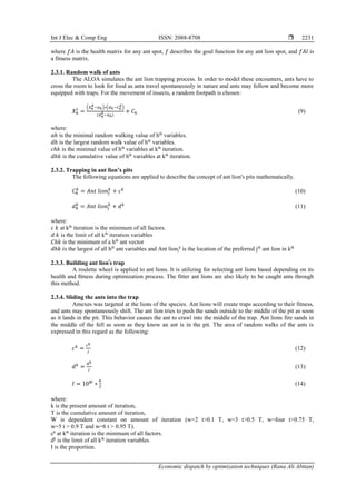
The necessary data required in ED [25], [27]. The units generating limits are presented in Table 1.
Also, the averaged B-coefficients for the power demands under study are presented in Table 2.
Table 1. Fuel cost function parameters
Unit No.
Fuel Cost Coefficients Generation Limits
A ($/MW) b ($/MWh) C ($/h) Pmin (MW) Pmax (MW)
1 0.03546 38.30553 1243.531 35 210
2 0.02111 36.32782 1658.5696 130 325
3 0.01799 38.27041 1356.6592 125 315
Table 2. The B-coefficients
B-coefficients=
0.000071 0.000030 0.000025
0.000030 0.000069 0.000032
0.000025 0.000032 0.000080
4.1.1. Ant lion optimization algorithm (ALOA)
The test device contains 3-generation systems with differing demands of 300-700 MW. The ALOA
approach is being applied for economic dispatches. Table 3 reports the division of the groups.
Table 3. Economic dispatch results, 3-unit system using ALOA method
Load P1 P2 P3 PL Total cost (fuel cost)
400 82.0783 174.9937 150.4959 7.56812 20812.2934
500 105.8799 212.7279 193.3064 11.9143 25465.4690
600 130.0210 250.84619 236.4367 17.3040 30333.9856
700 154.5139 289.3596 279.8944 23.7680 35424.391
Note: load P1, P2 and P2 for MW- total cost for $/h
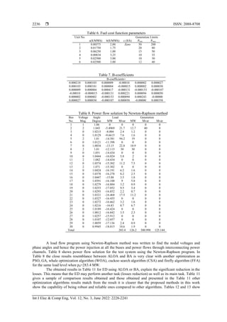
4.1.2. Bat algorithm (BA)
In this scenario, the BA is devised to deal with complex equations as bats have a good ability to
forage in order to survive, and the ant lion method simulates the evolution of a group of lions, which divide
into groups and share information in order to obtain the shortest and best path. Table 4 shows the results
obtained for economic dispatch using BA method. The results of Table 4 is close to these of Table 3,
particularly at the 400-700 MW load level. The ant lion optimization and bat algorithm methods are first used
to find the optimal economic dispatch of a well-documented systems. Three standard systems were
considered [11], [27]–[29]. Table 5 shows the here used ALOA and BA methods results along with other
optimization algorithms for comparison to validate the effectiveness of the introduced methods and verify the
validity of the ant lion optimization and bat algorithm adopted in this work. Table 5 presents a sample
comparison result selected from literature and those obtained in this work for 400 to 700MW load case. The
results concerned are P1, P2, P3, PL and total cost (fuel cost) as those are the new considered factors here.
The results resemblance is quite evident between these obtained in this work and those documented in the
literature as noted. This scenario is the first, as there will be another investigation that will apply other
techniques such as a genetic algorithm [30], [31].
Table 4. Economic dispatch results, 3-unit system using BA method
Load P1 P2 P3 PL Total cost (fuel cost)
400 82.07835 174.9937 150.4960 7.5681254 20812.2934
500 105.8799 212.7279 193.3064 11.9143 25465.4690
600 130.0210 250.8462 236.4367 17.3040 30333.9856
700 152.8146 291.0264 279.9525 23.7936 35424.4149
Note: load P1, P2 and P2 for MW- total cost for $/h

8. Int J Elec & Comp Eng ISSN: 2088-8708 
Economic dispatch by optimization techniques (Rana Ali Abttan)
2235
Table 5. Comparing ALOA and BA methods to other optimization algorithms for 3 generator system
pD Performance ALO BA GA [28] PSO [28] TS [29] ABC [12] CSA [32]
400 P1 (MW) 82.0783 82.0783 102.617 102.612 104.0372 102.5422
P2 (MW) 174.9937 174.9937 153.825 153.809 150.0000 153.7333
P3 (MW) 150.4959 150.4960 151.011 150.991 153.3721 151.1370
PL (MW) 7.56812 7.56812 7.41324 7.41173 7.4093 7.568
Total cost (fuel cost) $/h 20812.2934 20812.2934 20840.1 20818.3 20845 20838 20812.3
500 P1 (MW) 105.8799 105.8799 128.997 128.984 181.4774 128.8241
P2 (MW) 212.7279 212.7279 192.683 192.645 150.0000 192.5837
P3 (MW) 193.3064 193.3064 190.11 190.063 180.0000 190.2859
PL (MW) 11.9143 11.9143 11.6964 11.6919 11.4774 11.6937
Total cost (fuel cost) $/h 25465.4690 25465.4690 25499.4 25495 25774 25495 25465.5
600 P1 (MW) 130.0210 130.0210 155.714 155.711 228.8856 NONE
P2 (MW) 250.84619 250.8462 231.895 231.859 178.8856
P3 (MW) 236.4367 236.4367 229.479 229.428 208.8856
PL (MW) 17.3040 17.3040 17.0039 16.9987 16.6568
Total cost (fuel cost) $/h 30333.9856 30333.9856 30372.3 30368.2 30837 30334.0
700 P1 (MW) 154.5139 152.8146 182.783 182.806 264.2929 182.6011
P2 (MW) 289.3596 291.0264 271.478 271.463 214.2929 271.2813
P3 (MW) 279.8944 279.9525 269.132 269.039 244.2929 269.4840
PL (MW) 23.7680 23.7936 23.365 23.3626 22.8788 23.3664
Total cost (fuel cost) $/h 35424.391 35424.4149 35466 35464.6 36037 35464 35424.4
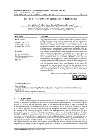
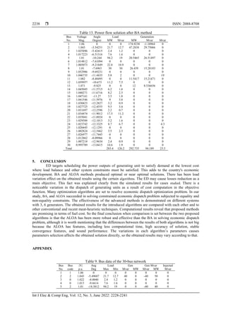
4.2. The six generating units test system
The method mentioned is extended to the IEEE test network, which consists of 30 buses, 6 thermal
generator units 41, as shown in Figure 1. Table 6 show the fuel cost and Table 7 presents the averaged
B-coefficients. Also, in Table 8 show the units generating limits are presented with the system data contained
in Table 9 and Table 10 (see in appendix).
Figure 1. Single line diagram of IEEE 30-bus test system

9.  ISSN: 2088-8708
Int J Elec & Comp Eng, Vol. 12, No. 3, June 2022: 2228-2241
2236
Table 6. Fuel cost function parameters
Unit No. Generation Limits
a($/MWh) b($/MWh) c ($/h) Pmin Pmax
1 0.00375 2.00 Zero 50 200
2 0.01750 1.75 20 80
3 0.06250 1.00 15 50
4 0.00834 3.25 10 35
5 0.02500 3.00 10 30
6 0.02500 3.00 12 40
Table 7. B-coefficients
B-coefficients=
0.000218 0.000103 0.000009 -0.00010 0.000002 0.000027
0.000103 0.000181 0.000004 -0.000015 0.000002 0.000030
0.000009 0.000004 0.000417 -0.000131 -0.000153 -0.000107
-0.00010 -0.000015 -0.000131 0.000221 0.000094 0.000050
0.000002 0.000002 -0.000153 0.000094 0.000243 -0.00000
0.000027 0.000030 -0.000107 0.000050 -0.00000 0.000358
Table 8. Power flow solution by Newton-Raphson method
Bus Voltage Angle Load Generation
No. Mag. Degree MW Mvar MW Mvar Mvar
1 1 1.06 0 0 0 0 0
2 2 1.043 -5.4969 21.7 12.7 40 0
3 0 1.0215 -8.004 2.4 1.2 0 0
4 0 1.0129 -9.6615 7.6 1.6 0 0
5 2 1.01 -14.381 94.2 19 0 0
6 0 1.0121 -11.398 0 0 0 0
7 0 1.0034 -13.15 22.8 10.9 0 0
8 2 1.01 -12.115 30 30 0 0
9 0 1.051 -14.434 0 0 0 0
10 0 1.0444 -16.024 5.8 2 0 0
11 2 1.082 -14.434 0 0 0 0
12 0 1.0574 -15.302 11.2 7.5 0 0
13 2 1.071 -15.302 0 0 0 0
14 0 1.0424 -16.191 6.2 1.6 0 0
15 0 1.0378 -16.278 8.2 2.5 0 0
16 0 1.0447 -15.88 3.5 1.8 0 0
17 0 1.0391 -16.188 9 5.8 0 0
18 0 1.0279 -16.884 3.2 0.9 0 0
19 0 1.0253 -17.052 9.5 3.4 0 0
20 0 1.0293 -16.852 2.2 0.7 0 0
21 0 1.0321 -16.468 17.5 11.2 0 0
22 0 1.0327 -16.455 0 0 0 0
23 0 1.0272 -16.662 3.2 1.6 0 0
24 0 1.0216 -16.83 8.7 6.7 0 0
25 0 1.0189 -16.424 0 0 0 0
26 0 1.0012 -16.842 3.5 2.3 0 0
27 0 1.0257 -15.912 0 0 0 0
28 0 1.0107 -12.057 0 0 0 0
29 0 1.0059 -17.136 2.4 0.9 0 0
30 0 0.9945 -18.015 10.6 1.9 0 0
Total 283.4 126.2 300.998 125.144
A load flow program using Newton-Raphson method was written to find the nodal voltages and
phase angles and hence the power injection at all the buses and power flows through interconnecting power
channels. Table 8 shows power flow solution for the test system using the Newton-Raphson program. In
Table 8 the close results resemblance between ALOA and BA is very clear with another optimization as
PSO, GA, whale optimization algorithm (WOA), cuckoo search algorithm (CSA) and firefly algorithm (FFA)
for the same load level when pd=283.4 MW.
The obtained results in Table 11 for ED using ALOA or BA, explain the significant reduction in the
losses. This means that the ED may perform another task (losses reduction) as well as its main task. Table 11
gives a sample of comparison results obtained and those obtained and presented in the Table 11 other
optimization algorithms results match from the result it is clearer that the proposed methods in this work
show the capability of being robust and reliable ones compared to other algorithms. Tables 12 and 13 show

10. Int J Elec & Comp Eng ISSN: 2088-8708 
Economic dispatch by optimization techniques (Rana Ali Abttan)
2237
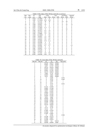
power flow solution for the test system using the Newton-Raphson program after ALOA and BA methods for
PD=283.4. Regarding the comparison between the BA and ALOA results in our study for this system, we can
get that the ant lion optimization is superior to that of bat algorithm.
Table 11. ALOA and BA methods results along with other optimization algorithms
pD Performance ALOA BA WOA [18] GA [33] PSO [34] CSA [35] FFA [35]
283.4 P1 (MW) 173.7835 173.78866 120.41 149.52
P2 (MW) 47.2827 47.2838 20.57 48.65
P3 (MW) 20.5462 20.5465 50.00 23.41
P4(MW) 26.4363 26.4390 35.00 22.26
P5 (MW) 11.5409 11.5417 24.97 19.88
P6 (MW) 12.0000 12.0000 40.00 27.23
PL (MW) 8.1895 8.189937 7.54 7.54
Total cost
(fuel cost) $/h
798.9175 798.95344 819.81 973.01
350 P1 (MW) 199.9999 199.9999 NONE
P2 (MW) 59.8850 55.6802
P3 (MW) 24.7492 23.4771
P4(MW) 35 35
P5 (MW) 21.5781 30
P6 (MW) 20.0724 16.8859
PL (MW) 11.2849 11.0434
Total cost
(fuel cost) $/h
1051.22094 1053.8739
400 P1 (MW) 200 199.9999 NONE
P2 (MW) 80 79.8067
P3 (MW) 31.9075 31.3746
P4(MW) 35 35
P5 (MW) 30 29.9999
P6 (MW) 36.3985 37.13710
PL (MW) 13.3061 13.3185
Total cost
(fuel cost) $/h
1276.3219 1276.3758
Table 12. Power flow solution after ALOA method
Bus Voltage Angle Load Generation
No. Mag. Degree MW Mvar MW Mvar Mvar
1 1.06 0 0 0 174.929 -1.11077 0
2 1.043 -3.54263 21.7 12.7 47.2827 29.75173 0
3 1.025495 -5.42431 2.4 1.2 0 0 0
4 1.017223 -6.51335 7.6 1.6 0 0 0
5 1.01 -10.2442 94.2 19 20.5462 26.51513 0
6 1.014812 -7.61117 0 0 0 0 0
7 1.005073 -9.21871 22.8 10.9 0 0 0
8 1.01 -7.6966 30 30 26.4363 15.28295 0
9 1.052985 -9.6926 0 0 0 0 0
10 1.046735 -11.4437 5.8 2 0 0 19
11 1.082 -8.48532 0 0 11.5409 15.21475 0
12 1.059957 -10.6732 11.2 7.5 0 0 0
13 1.071 -9.82523 0 0 12 8.536679 0
14 1.045045 -11.5717 6.2 1.6 0 0 0
15 1.040271 -11.6718 8.2 2.5 0 0 0
16 1.047161 -11.2702 3.5 1.8 0 0 0
17 1.041545 -11.5978 9 5.8 0 0 0
18 1.030423 -12.283 3.2 0.9 0 0 0
19 1.027725 -12.4557 9.5 3.4 0 0 0
20 1.031696 -12.2598 2.2 0.7 0 0 0
21 1.034474 -11.9015 17.5 11.2 0 0 0
22 1.035041 -11.8927 0 0 0 0 0
23 1.029588 -12.1015 3.2 1.6 0 0 0
24 1.023741 -12.3328 8.7 6.7 0 0 4.3
25 1.020445 -12.1293 0 0 0 0 0
26 1.002823 -12.5464 3.5 2.3 0 0 0
27 1.026977 -11.7448 0 0 0 0 0
28 1.012862 -8.09991 0 0 0 0 0
29 1.007218 -12.9656 2.4 0.9 0 0 0
30 0.995789 -13.8417 10.6 1.9 0 0 0
Total 283.4 126.2 292.735 94.19 23.3

11.  ISSN: 2088-8708
Int J Elec & Comp Eng, Vol. 12, No. 3, June 2022: 2228-2241
2238
Table 13. Power flow solution after BA method
Bus Voltage Angle Load Generation
No. Mag. Degree MW Mvar MW Mvar Mvar
1 1.06 0 0 0 174.9238 -1.10964 0
2 1.043 -3.54251 21.7 12.7 47.2838 29.75066 0
3 1.025496 -5.42415 2.4 1.2 0 0 0
4 1.017223 -6.51316 7.6 1.6 0 0 0
5 1.01 -10.244 94.2 19 20.5465 26.51497 0
6 1.014812 -7.61094 0 0 0 0 0
7 1.005073 -9.21849 22.8 10.9 0 0 0
8 1.01 -7.6963 30 30 26.439 15.28183 0
9 1.052986 -9.69231 0 0 0 0 0
10 1.046735 -11.4435 5.8 2 0 0 19
11 1.082 -8.48495 0 0 11.5417 15.21471 0
12 1.059957 -10.673 11.2 7.5 0 0 0
13 1.071 -9.825 0 0 12 8.536656 0
14 1.045045 -11.5715 6.2 1.6 0 0 0
15 1.040271 -11.6716 8.2 2.5 0 0 0
16 1.047161 -11.27 3.5 1.8 0 0 0
17 1.041546 -11.5976 9 5.8 0 0 0
18 1.030423 -12.2827 3.2 0.9 0 0 0
19 1.027725 -12.4555 9.5 3.4 0 0 0
20 1.031697 -12.2596 2.2 0.7 0 0 0
21 1.034474 -11.9012 17.5 11.2 0 0 0
22 1.035041 -11.8924 0 0 0 0 0
23 1.029588 -12.1013 3.2 1.6 0 0 0
24 1.023742 -12.3325 8.7 6.7 0 0 4.3
25 1.020445 -12.1291 0 0 0 0 0
26 1.002824 -12.5462 3.5 2.3 0 0 0
27 1.026977 -11.7445 0 0 0 0 0
28 1.012862 -8.09966 0 0 0 0 0
29 1.007218 -12.9654 2.4 0.9 0 0 0
30 0.995789 -13.8415 10.6 1.9 0 0 0
Total 283.4 126.2 292.735 94.189 23.3
5. CONCLUSION
ED targets scheduling the power outputs of generating unit to satisfy demand at the lowest cost
where load balance and other system constraints must be satisfied. This adds to the country's economic
development. BA and ALOA methods produced optimal or near optimal solutions. There has been load
variation effect on the obtained results using the certain algorithms. The ED may cause losses reduction as a
main objective. This fact was explained clearly from the simulated results for cases studied. There is a
noticeable variation in the dispatch of generating units as a result of cost computation in the objective
function. Many optimization algorithms are set to resolve economic dispatch optimization problem. In our
study, BA, and ALOA succeeded in solving constrained economic dispatch problem subjected to equality and
non-equality constraints. The effectiveness of the advanced methods is demonstrated on different systems
with 3, 6 generators. The obtained results for the introduced algorithms are compared with each other and to
other conventional and recent meat-heuristic techniques. Computational results reveal that proposed methods
are promising in terms of fuel cost. So the final conclusion when comparison is set between the two proposed
algorithms is that the ALOA has been more robust and effective than the BA in solving economic dispatch
problem, although it is worth mentioning that the differences between the results of both algorithms is not big
because the ALOA has features, including less computational time, high accuracy of solution, stable
convergence features, and sound performance. The variations in each algorithm’s parameters causes
parameters selection affects the obtained solution directly, so the obtained results may vary according to that.
APPENDIX
Table 9. Bus data of the 30-bus network
Bus Bus |V| Ang Load Gen Gen Mvar Injected
No. code p.u. Deg Max Min Mvar MW Mvar MW Mvar
1 1 1.06 0 0 0 0 0 0 0 0
2 2 1.043 -5.49687 21.7 12.7 40 0 -40 50 0
3 0 1.022 -8.0040 2.4 1.2 0 0 0 0 0
4 0 1.013 -9.6614 7.6 1.6 0 0 0 0 0
5 2 1.01 -14.3812 94.2 19 0 0 -40 40 0

12. Int J Elec & Comp Eng ISSN: 2088-8708 
Economic dispatch by optimization techniques (Rana Ali Abttan)
2239
Table 9. Bus data of the 30-bus network (continue)
Bus Bus |V| Ang Load Gen Gen Mvar Injected
No. code p.u. Deg Max Min Mvar MW Mvar MW Mvar
6 0 1.012 -11.3979 0 0 0 0 0 0 0
7 0 1.003 -13.14950 22.8 10.9 0 0 0 0 0
8 2 1.01 -12.1153 30 30 0 0 -10 60 0
9 0 1.051 -14.4338 0 0 0 0 0 0 0
10 0 1.044 -16.0241 5.8 2 0 0 -6 24 19
11 2 1.082 -14.4338 0 0 0 0 0 0 0
12 0 1.057 -15.3024 11.2 7.5 0 0 0 0 0
13 2 1.071 -15.3024 0 0 0 0 -6 24 0
14 0 1.042 -16.1913 6.2 1.6 0 0 0 0 0
15 0 1.038 -16.2782 8.2 2.5 0 0 0 0 0
16 0 1.045 -15.8804 3.5 1.8 0 0 0 0 0
17 0 1.039 -16.18829 9 5.8 0 0 0 0 0
18 0 1.028 -16.8835 3.2 0.9 0 0 0 0 0
19 0 1.025 -17.0519 9.5 3.4 0 0 0 0 0
20 0 1.029 -16.8522 2.2 0.7 0 0 0 0 0
21 0 1.032 -16.4684 17.5 11.2 0 0 0 0 0
22 0 1.033 -16.4546 0 0 0 0 0 0 0
23 0 1.027 -16.6623 3.2 1.6 0 0 0 0 0
24 0 1.022 -16.8301 8.7 6.7 0 0 0 0 4.3
25 0 1.019 -16.4238 0 0 0 0 0 0 0
26 0 1.001 -16.8422 3.5 2.3 0 0 0 0 0
27 0 1.026 -15.9124 0 0 0 0 0 0 0
28 0 1.011 -12.0574 0 0 0 0 0 0 0
29 0 1.006 -17.1363 2.4 0.9 0 0 0 0 0
30 0 0.995 -18.0146 10.6 1.9 0 0 0 0 0
Table 10. Line data of the 30-bus network
Bus No. Bus No. R1 X1 B/2 Tap at bus
1 2 0.0192 0.0575 0.0264 1
1 3 0.0452 0.1852 0.0204 1
2 4 0.057 0.1737 0.0184 1
3 4 0.0132 0.0379 0.0042 1
2 5 0.0472 0.1983 0.0209 1
2 6 0.0581 0.1763 0.0187 1
4 6 0.0119 0.0414 0.0045 1
5 7 0.046 0.116 0.0102 1
6 7 0.0267 0.082 0.0085 1
6 8 0.012 0.042 0.0045 1
6 9 0 0.208 0 0.978
6 10 0 0.556 0 0.969
9 11 0 0.208 0 1
9 10 0 0.11 0 1
4 12 0 0.256 0 0.932
12 13 0 0.14 0 1
12 14 0.1231 0.2559 0 1
12 15 0.0662 0.1304 0 1
12 16 0.0945 0.1987 0 1
14 15 0.221 0.1997 0 1
16 17 0.0824 0.1923 0 1
15 18 0.1073 0.2185 0 1
18 19 0.0639 0.1292 0 1
19 20 0.034 0.068 0 1
10 20 0.0936 0.209 0 1
10 17 0.0324 0.0845 0 1
10 21 0.0348 0.0749 0 1
10 22 0.0727 0.1499 0 1
21 22 0.0116 0.0236 0 1
15 23 0.1 0.202 0 1
22 24 0.115 0.179 0 1
23 24 0.132 0.27 0 1
24 25 0.1885 0.3292 0 1
25 26 0.2544 0.38 0 1
25 27 0.1093 0.2087 0 1
28 27 0 0.396 0 0.968
27 29 0.2198 0.4153 0 1
27 30 0.3202 0.6027 0 1
29 30 0.2399 0.4533 0 1
8 28 0.0636 0.2 0.0214 1
6 28 0.0169 0.0599 0.065 1

13.  ISSN: 2088-8708
Int J Elec & Comp Eng, Vol. 12, No. 3, June 2022: 2228-2241
2240
REFERENCES
[1] A. J. Wood, B. F. Wollenberg, and G. B. Sheblé, Power generation, operation and control, vol. 39, no. 5. John Wiley & Sons,
2014.
[2] B. H. Chowdhury and S. Rahman, “A review of recent advances in economic dispatch,” IEEE Transactions on Power Systems,
vol. 5, no. 4, pp. 1248–1259, 1990, doi: 10.1109/59.99376.
[3] M. M. Mijwil and R. A. Abttan, “Artificial intelligence: a survey on evolution and future trends,” Asian Journal of Applied
Sciences, vol. 9, no. 2, Apr. 2021, doi: 10.24203/ajas.v9i2.6589.
[4] K. Y. Lee and A. Sode-Yome, “Adaptive hopfield neural networks for economic load dispatch,” IEEE Transactions on Power
Systems, vol. 13, no. 2, pp. 519–526, May 1998, doi: 10.1109/59.667377.
[5] C. T. Su and C. T. Lin, “New approach with a Hopfield modeling framework to economic dispatch,” IEEE Transactions on
Power Systems, vol. 15, no. 2, pp. 541–545, May 2000, doi: 10.1109/59.867138.
[6] W. M. Lin, F. S. Cheng, and M. T. Tsay, “Nonconvex economic dispatch by integrated artificial intelligence,” IEEE Transactions
on Power Systems, vol. 16, no. 2, pp. 307–311, May 2001, doi: 10.1109/59.918303.
[7] H. Altun and T. Yalcinoz, “Implementing soft computing techniques to solve economic dispatch problem in power systems,”
Expert Systems with Applications, vol. 35, no. 4, pp. 1668–1678, Nov. 2008, doi: 10.1016/j.eswa.2007.08.066.
[8] K. B. Sahay, A. Sonkar, and A. Kumar, “Economic load dispatch using genetic algorithm optimization technique,” Oct. 2019, doi:
10.23919/ICUE-GESD.2018.8635729.
[9] T. Niknam, F. Golestane, and B. Bahmanifirouzi, “Modified adaptive PSO algorithm to solve dynamic economic dispatch,” in
PEAM 2011 - Proceedings: 2011 IEEE Power Engineering and Automation Conference, Sep. 2011, vol. 1, pp. 108–111, doi:
10.1109/PEAM.2011.6134807.
[10] G. Abbas, J. Gu, U. Farooq, A. Raza, M. U. Asad, and M. E. El-Hawary, “Solution of an economic dispatch problem through
particle swarm optimization: a detailed survey - part ii,” IEEE Access, vol. 5, pp. 24426–24445, 2017, doi:
10.1109/ACCESS.2017.2768522.
[11] X. Chen, B. Xu, and W. Du, “An improved particle swarm optimization with biogeography-based learning strategy for economic
dispatch problems,” Complexity, vol. 2018, pp. 1–15, Jul. 2018, doi: 10.1155/2018/7289674.
[12] G. P. Dixit, H. M. Dubey, M. Pandit, and B. K. Panigrahi, “Artificial bee colony optimization for combined economic load and
emission dispatch,” in International Conference on Sustainable Energy and Intelligent Systems (SEISCON 2011), 2011,
pp. 340–345, doi: 10.1049/cp.2011.0386.
[13] R. K. Rao, P. Srinivas, M. S. M. Divakar, and G. S. N. M. Venkatesh, “Artificial bee colony optimization for multi objective
economic load dispatch of a modern power system,” in 2016 International Conference on Electrical, Electronics, and
Optimization Techniques (ICEEOT), Mar. 2016, pp. 4097–4100, doi: 10.1109/ICEEOT.2016.7755486.
[14] S. Ma, Y. Wang, and Y. Lv, “Multiobjective environment/economic power dispatch using evolutionary multiobjective
optimization,” IEEE Access, vol. 6, pp. 13066–13074, 2018, doi: 10.1109/ACCESS.2018.2795702.
[15] M. Basu and A. Chowdhury, “Cuckoo search algorithm for economic dispatch,” Energy, vol. 60, pp. 99–108, Oct. 2013, doi:
10.1016/j.energy.2013.07.011.
[16] Z. Zakaria, T. K. A. Rahman, and E. E. Hassan, “Economic load dispatch via an improved bacterial foraging optimization,” in
2014 IEEE 8th International Power Engineering and Optimization Conference (PEOCO2014), Mar. 2014, pp. 380–385, doi:
10.1109/PEOCO.2014.6814458.
[17] A. S. Reddy and K. Vaisakh, “Shuffled differential evolution for large scale economic dispatch,” Electric Power Systems
Research, vol. 96, pp. 237–245, Mar. 2013, doi: 10.1016/j.epsr.2012.11.010.
[18] H. J. Touma, “Study of the economic dispatch problem on IEEE 30-bus system using whale optimization algorithm,”
International Journal of Engineering Technology and Sciences, vol. 3, no. 1, pp. 11–18, Jun. 2016, doi:
10.15282/ijets.5.2016.1.2.1041.
[19] Y. V. K. Reddy and M. D. Reddy, “Flower pollination algorithm to solve dynamic economic loading of units with piecewise fuel
options,” Indonesian Journal of Electrical Engineering and Computer Science, vol. 16, no. 1, pp. 9–16, Oct. 2019, doi:
10.11591/ijeecs.v16.i1.pp9-16.
[20] M. Y. Nassar, M. N. Abdullah, and A. A. Rahimoon, “Optimal economic dispatch of power generation solution using lightning
search algorithm,” IAES International Journal of Artificial Intelligence (IJ-AI), vol. 9, no. 3, pp. 371–378, Sep. 2020, doi:
10.11591/ijai.v9.i3.pp371-378.
[21] N. A. M. Kamari, M. A. Zulkifley, N. F. Ramli, and I. Musirin, “Optimal power scheduling for economic dispatch using moth
flame optimizer,” Indonesian Journal of Electrical Engineering and Computer Science, vol. 20, no. 1, pp. 379–384, Oct. 2020,
doi: 10.11591/ijeecs.v20.i1.pp379-384.
[22] P. T. Ha, H. M. Hoang, T. T. Nguyen, and T. T. Nguyen, “Modified moth swarm algorithm for optimal economic load dispatch
problem,” TELKOMNIKA (Telecommunication Computing Electronics and Control), vol. 18, no. 4, pp. 2140–2147, Aug. 2020,
doi: 10.12928/telkomnika.v18i4.15032.
[23] S. Bhongade and S. Agarwal, “Artificial bee colony algorithm for an optimal solution for combined economic and emission
dispatch problem,” International Journal of Applied Power Engineering (IJAPE), vol. 5, no. 3, pp. 111–119, Dec. 2016, doi:
10.11591/ijape.v5.i3.pp111-119.
[24] S. Mirjalili, “The ant lion optimizer,” Advances in Engineering Software, vol. 83, pp. 80–98, May 2015, doi:
10.1016/j.advengsoft.2015.01.010.
[25] F. Z. Alazemi and A. Y. Hatata, “Ant lion optimizer for optimum economic dispatch considering demand response as a visual
power plant,” Electric Power Components and Systems, vol. 47, no. 6–7, pp. 629–643, Apr. 2019, doi:
10.1080/15325008.2019.1602799.
[26] X. S. Yang and X. He, “Bat algorithm: literature review and applications,” International Journal of Bio-Inspired Computation,
vol. 5, no. 3, 2013, doi: 10.1504/IJBIC.2013.055093.
[27] Y. A. Gherbi, H. Bouzeboudja, and F. Lakdja, “Economic dispatch problem using bat algorithm,” Leonardo Journal of Sciences,
no. 24, pp. 75–84, 2014.
[28] A. L. Devi and O. V. Krishna, “Combined economic and emission dispatch using evolutionary algorithms-a case study,” ARPN
Journal of Engineering and Applied Sciences, vol. 3, no. 6, pp. 28–35, 2008.
[29] K. Senthil and K. Manikandan, “Improved tabu search algorithm to economic emission dispatch with transmission line
constraint,” Search, vol. 1, no. 2, pp. 145–149, 2010.
[30] M. M. Mijwil and R. A. Abttan, “Applying genetic algorithm to optimization second-order bandpass MGMFB filter,” Pertanika
Journal of Science and Technology, vol. 28, no. 4, pp. 1413–1425, Oct. 2020, doi: 10.47836/pjst.28.4.15.

14. Int J Elec & Comp Eng ISSN: 2088-8708 
Economic dispatch by optimization techniques (Rana Ali Abttan)
2241
[31] M. M. Mijwil and R. A. Abttan, “Utilizing the genetic algorithm to pruning the C4.5 decision tree algorithm,” Asian Journal of
Applied Sciences, vol. 9, no. 1, Feb. 2021, doi: 10.24203/ajas.v9i1.6503.
[32] Z. M. Yasin, N. F. A. Aziz, N. A. Salim, N. A. Wahab, and N. A. Rahmat, “Optimal economic load dispatch using multiobjective
cuckoo search algorithm,” Indonesian Journal of Electrical Engineering and Computer Science, vol. 12, no. 1, pp. 168–174, Oct.
2018, doi: 10.11591/ijeecs.v12.i1.pp168-174.
[33] L. A. Koridak, M. Rahli, and M. Younes, “Hybrid optimization of the emission and economic dispatch by the genetic algorithm,”
Leonardo Journal of Sciences, vol. 8, no. 14, pp. 193–203, 2008.
[34] P. A.-D.-V. Raj, T. G. Palanivelu, and R. Gnanadass, “Optimal power flow solution for combined economic emission dispatch
problem using particle swarm optimization technique,” Journal of Electrical Systems, vol. 3, no. 1, pp. 13–25, 2007.
[35] N. Karthik, A. K. Parvathy, and R. Arul, “Non-convex economic load dispatch using cuckoo search algorithm,” Indonesian
Journal of Electrical Engineering and Computer Science, vol. 5, no. 1, pp. 48–57, Jan. 2017, doi: 10.11591/ijeecs.v5.i1.pp48-57.
BIOGRAPHIES OF AUTHORS
Rana Ali Abttan received the B.Sc, M.Sc. and PhD degrees in Electrical
Engineering from the University of Technology (UOT), Baghdad, Iraq, in 2008, 2011 and
2019, respectively. Currently, she is a Lecturer and an academic member of staff in the
computer techniques engineering department at Baghdad college of economic sciences
university, in Iraq. She graduated from Publons academy as a peer reviewer. Her research
interests include renewable energy, power system operation, power system stability, power
system maintenance, power generation, power grids, power supply quality, hydroelectric
power stations, load flow control, power transmission lines, power transmission planning,
power transmission protection, power transmission reliability, circuit breakers, relay
protection, harmonic distortion, overcurrent protection, power distribution protection, power
electronics, network reliability, distributed generation, distribution network reconfiguration,
and applications of artificial intelligence and computational algorithms in power system. She
can be contacted at email: rana.ali.abttan@baghdadcollege.edu.iq.
Adnan Hasan Tawafan was born in Kerbala, Iraq, in 1971. He received the M.S.
degree in electrical engineering from University of Technology, Baghdad, Iraq in 2002, and
the Ph.D. degree in electrical engineering from UTeM, Malaysia in 2014. Since 2005, he has
been with electrical technical department in Technical Institute of Karbala, Iraq. His research
interests concern: analysis and design of distribution system, protection, power quality
improvement, power electronics applications and risk management. Email address:
inkr.adn@atu.edu.iq.
Samar Jaafar Ismael received the B.Sc, M.Sc. and PhD degrees in Electrical
Engineering from the University of Technology (UOT), Baghdad, Iraq, in 2000, 2003 and
2017, respectively. She is a staff member in Electromechanical Engineering (EME)
Department, the University of Technology since 2005. Along with academic job, Dr. Samar
currently occupying many positions such as the director of the graduate studies division since
2018, member of the committee for graduate studies examination since 2017, director of the
EME department's electronic website since 2017, member of the e-learning committee since
2018, and a member of the committee for the issuance of documents for graduate students.
She has finished the Google classroom training application course and become an e-learning
advisor in the EME Department. Also, Samar is a member of the syndicate of Iraqi engineers.
As far as her academic experience is concerned, Dr. Samar has many publications in electrical
engineering. Besides, she was a peer reviewer of the Engineering and Technology Journal and
reviewed many. Her research interests include power system analysis, artificial intelligence
algorithms, graph theory and electrical machines and aiming to develop many scientific fields,
especially in education. She can be contacted at email: 50240@uotechnology.edu.iq.