Superconductivity in MW circuits

1. arXiv:1007.1058v1[quant-ph]7Jul2010
The dynamical Casimir effect in superconducting microwave circuits
J.R. Johansson,1
G. Johansson,2
C.M. Wilson,2
and Franco Nori1, 3
1
Advanced Science Institute, RIKEN, Wako-shi, Saitama 351-0198, Japan
2
Microtechnology and Nanoscience, MC2, Chalmers University of Technology, SE-412 96 G¨oteborg, Sweden
3
Physics Department, The University of Michigan, Ann Arbor, Michigan 48109-1040, USA
(Dated: July 8, 2010)
We theoretically investigate the dynamical Casimir effect in electrical circuits based on supercon-
ducting microfabricated waveguides with tunable boundary conditions. We propose to implement
a rapid modulation of the boundary conditions by tuning the applied magnetic flux through super-
conducting quantum interference devices (SQUIDs) that are embedded in the waveguide circuits.
We consider two circuits: (i) An open waveguide circuit that corresponds to a single mirror in free
space, and (ii) a resonator coupled to a microfabricated waveguide, which corresponds to a single-
sided cavity in free space. We analyze the properties of the dynamical Casimir effect in these two
setups by calculating the generated photon-flux density, output-field correlation functions, and the
quadrature squeezing spectra. We show that these properties of the output field exhibit signatures
unique to the radiation due to the dynamical Casimir effect, and could therefore be used for dis-
tinguishing the dynamical Casimir effect from other types of radiation in these circuits. We also
discuss the similarities and differences between the dynamical Casimir effect, in the resonator setup,
and downconversion of pump photons in parametric oscillators.
PACS numbers: 85.25.Cp, 42.50.Lc, 84.40.Az
I. INTRODUCTION
Quantum field theory predicts that photons can be cre-
ated from vacuum fluctuations when the boundary con-
ditions of the field are time-dependent. This effect, of-
ten called the dynamical Casimir effect, was predicted by
G.T. Moore [1] in 1970, in the context of a cavity com-
prised of two moving ideal mirrors. In 1976, S.A. Fulling
et al. [2] showed that a single mirror in free space also
generates radiation, when subjected to a nonuniform ac-
celeration. The role of the moving mirrors in these stud-
ies is to impose time-dependent boundary conditions on
the electromagnetic fields. The interaction between the
time-dependent boundary condition and the zero-point
vacuum fluctuations can result in photon creation, for a
sufficiently strong time-dependence [3–6].
However, it has proven to be a difficult task to ex-
perimentally observe the dynamical Casimir effect. The
problem lies in the difficulty in changing the boundary
conditions, e.g., by moving physical objects, such as mas-
sive mirrors, sufficiently fast to generate a significant
number of photons. Although there are proposals (see,
e.g., Ref. [7]) for experimentally observing the dynami-
cal Casimir effect using massive mirrors, no experimental
verification of the dynamical Casimir effect has been re-
ported to date [5]. In order to circumvent this difficulty
a number of theoretical proposals have suggested to use
experimental setups where the boundary conditions are
modulated by some effective motion instead. Examples
of such proposals include to use lasers to modulate the re-
flectivity of thin semiconductor films [8, 9] or to modulate
the resonance frequency of a superconducting stripline
resonator [10], to use a SQUID to modulate the bound-
ary condition of a superconducting waveguide [11], and
to use laser pulses to rapidly modulate the vacuum Rabi
frequency in cavity QED systems [12, 13].
In this paper we investigate manifestations of the
dynamical Casimir effect in superconducting electrical
circuits based on microfabricated (including coplanar)
waveguides. Recent theoretical and experimental de-
velopments in the field of superconducting electronics,
which to a large extent is driven by research on quan-
tum information processing [14–16], include the realiza-
tion of strong coupling between artificial-atoms and os-
cillators [17–19] (so called circuit QED), studies of the
ultra-strong coupling regime in circuit QED [20], single-
artificial-atom lasing [21, 22], Fock-state generation and
state tomography [23, 24]. Also, there has recently been
an increased activity in studies of multimode quantum
fields in superconducting circuits, both theoretically and
experimentally, see e.g., Refs. [25–28], and in experimen-
tal work on frequency-tunable resonators [29–32]. These
studies exemplify how quantum-optics-like systems can
be implemented in superconducting electrical circuits
[33], where waveguides and resonators play the roles of
light beams and cavities, and Josephson-junction based
artificial atoms play the role of natural atoms in the orig-
inal quantum optics setups.
Here, we theoretically investigate the possibility to ex-
ploit these recent advances to realize a system [11] where
the dynamical Casimir effect can be observed experimen-
tally in an electrical circuit. We consider two circuit
configurations, see Fig. 1(c)-(d), for which we study the
dynamical Casimir effect in the broadband and narrow-
band limits, respectively. We analyze the properties of
the radiation due to the dynamical Casimir effect in these
systems, and we identify a number of signatures in exper-
imentally measurable signals that could be used to distin-
guish the radiation due to the dynamical Casimir effect
from other types of radiation, such as thermal noise.

2. 2
FIG. 1. (color online) Schematic illustration of the dynamical Casimir effect, in the case of a single oscillating mirror in free
space (a), and in the case of a cavity in free space, where the position of one of the mirrors oscillates (b). In both cases, photons
are generated due to the interplay between the time-dependent boundary conditions imposed by the moving mirrors, and the
vacuum fluctuations. Here, Ω is the frequency of the oscillatory motion of the mirrors, and a is the amplitude of oscillations.
The dynamical Casimir effect can also be studied in electrical circuits. Two possible circuit setups that correspond to the
quantum-optics setups (a) and (b) are shown schematically in (c) and (d), respectively. In these circuits, the time-dependent
boundary condition imposed by the SQUID corresponds to the motion of the mirrors in (a) and (b).
The dynamical Casimir effect has also previously been
discussed in the context of superconducting electrical
circuits in Ref. [34]. Another related theoretical pro-
posal to use superconducting electrical circuits to inves-
tigate photon creation due to nonadiabatic changes in
the field parameters was presented in [35], where a cir-
cuit for simulating the Hawking radiation was proposed.
In contrast to these works, here we exploit the demon-
strated fast tunability of the boundary conditions for a
one-dimensional electromagnetic field, achieved by termi-
nating a microfabricated waveguide with a SQUID [32].
(See, e.g., Ref. [36] for a review of the connections be-
tween the dynamical Casimir effect, the Unruh effect and
the Hawking effect).
This paper is organized as follows: In Sec. II, we briefly
review the dynamical Casimir effect. In Sec. III, we pro-
pose and analyze an electrical circuit, Fig. 1(c), based
on an open microfabricated waveguide, for realizing the
dynamical Casimir effect, and we derive the resulting
output field state. In Sec. IV, we propose and analyze
an alternative circuit, Fig. 1(d), featuring a waveguide
resonator. In Sec. V, we investigate various measure-
ment setups that are realizable in electrical circuits in
the microwave regime, and we explicitly evaluate the
photon-flux intensities and output-field correlation func-
tions for the two setups introduced in Sec. III and IV. In
Sec. VI, we explore the similarities between the dynami-
cal Casimir effect, in the resonator setup, and the closely
related parametric oscillator with a Kerr-nonlinearity.
Finally, a summary is given in Sec. VII.
II. BRIEF REVIEW OF THE DYNAMICAL
CASIMIR EFFECT
A. Static Casimir effect
Two parallel perfectly conducting uncharged plates
(ideal mirrors) in vacuum attract each other with a force
known as the Casimir force. This is the famous static
Casimir effect, predicted by H.B.G. Casimir in 1948 [37],
and it can be interpreted as originating from vacuum
fluctuations and due to the fact that the electromagnetic
mode density is different inside and outside of the cavity
formed by the two mirrors. The difference in the mode
density results in a radiation pressure on the mirrors,
due to vacuum fluctuations, that is larger from the out-
side than from the inside of the cavity, thus producing
a force that pushes the two mirrors towards each other.
The Casimir force has been thoroughly investigated theo-
retically, including different geometries, nonideal mirrors,
finite temperature, and it has been demonstrated exper-
imentally in a number of different situations (see, e.g.,
Refs. [41–43]). For reviews of the static Casimir effect,
see, e.g., Refs. [44–46].
B. Dynamical Casimir effect
The dynamical counterpart to the static Casimir effect
occurs when one or two of the mirrors move. The motion
of a mirror can create electromagnetic excitations, which
results in a reactive damping force that opposes the mo-

3. 3
Static Casimir Effect Dynamical Casimir Effect
Description Attractive force between two conductive plates in
vacuum.
Photon production due to a fast modulation of
boundary conditions.
Theory Casimir (1948) [37], Lifshitz (1956) [38]. Moore (1970) [1], Fulling et al. (1976) [2].
Experiment
Sparnaay (1958) [39], van Blokland et al.. (1978) [40],
Lamoreaux (1997) [41], Mohideen et al.. (1998) [42].
—
TABLE I. Brief summary of early work on the static and the dynamical Casimir effect. The static Casimir effect has been
experimentally verified, but experimental verification of the dynamical Casimir effect has not yet been reported [5].
tion of the mirror [47]. This prediction can be counter-
intuitive at first sight, because it involves the generation
of photons “from nothing” (vacuum) with uncharged con-
ducting plates, and it has no classical analogue. However,
in the quantum mechanical description of the electro-
magnetic field, even the vacuum contains fluctuations,
and the interaction between these fluctuations and the
time-dependent boundary conditions can create excita-
tions (photons) in the electromagnetic field. In this pro-
cess, energy is taken from the driving of the boundary
conditions to excite vacuum fluctuations to pairs of real
photons, which propagate away from the mirror.
The electromagnetic field in a one-dimensional cavity
with variable length was first investigated quantum me-
chanically by G.T. Moore [1], in 1970. In that seminal
paper, the exact solution for the electromagnetic field in
a one-dimensional cavity with an arbitrary cavity-wall
trajectory was given in terms of the solution to a func-
tional equation, known as Moore’s equation. Explicit
solutions to this equation for specific mirror motions has
been the topic of numerous subsequent papers, includ-
ing perturbative approaches valid in the short-time limit
[48], asymptotic solutions for the long-time limit [49], an
exact solution for a nearly-harmonically oscillating mir-
ror [50], numerical approaches [51], and renormalization
group calculations valid in both the short-time and long-
time limits [52, 53]. Effective Hamiltonian formulations
were reported in [54–56], and the interaction between the
cavity field and a detector was studied in [57, 58]. The
dynamical Casimir effect was also investigated in three-
dimensional cavities [57–59], and for different types of
boundary conditions [60, 61]. The rate of build-up of
photons depends in general on the exact trajectory of
the mirror, and it is also different in the one-dimensional
and the three-dimensional case. For resonant conditions,
i.e., where the mirror oscillates with twice the natural fre-
quency of the cavity, the number of photons in a perfect
cavity grows exponentially with time [62].
An alternative approach that focuses on the radiation
generated by a nonstationary mirror, rather than the
build-up of photons in a perfect cavity, was developed by
S.A. Fulling et al. [2], in 1976. In that paper, it was shown
that a single mirror in one-dimensional free space (vac-
uum) subjected to a nonuniform acceleration also pro-
duces radiation. The two cases of oscillatory motion of a
single mirror, and a cavity with walls that oscillate in a
synchronized manner, were studied in Refs. [63, 64], using
scattering analysis. The radiation from a single oscillat-
ing mirror was also analyzed in three dimensions [65].
Table I briefly compares the static and the dynamical
Casimir effect. See, e.g., Refs. [3–6] for extensive reviews
of the dynamical Casimir effect.
C. Photon production rate
The rate of photon production of an oscillating ideal
mirror in one-dimensional free space [63], see Fig. 1(a),
is, to first order,
N
T
=
Ω
3π
v
c
2
, (1)
where N is the number of photons generated during the
time T , Ω is the oscillation frequency of the mirror,
v = aΩ is the maximum speed of the mirror, and a is
the amplitude of the mirror’s oscillatory motion. From
this expression it is apparent that to achieve significant
photon production rates, the ratio v/c must not be too
small (see, e.g., Table II). The maximum speed of the
mirror must therefore approach the speed of light. The
spectrum of the photons generated in this process has a
distinct parabolic shape, between zero frequency and the
driving frequency Ω,
n(ω) ∝
a
c
2
ω(Ω − ω). (2)
This spectral shape is a consequence of the density
of states of electromagnetic modes in one-dimensional
space, and the fact that photons are generated in pairs
with frequencies that add up to the oscillation frequency
of the boundary: ω1 + ω2 = Ω.
By introducing a second mirror in the setup, so that a
cavity is formed, see Fig. 1(b), the dynamical Casimir ra-
diation can be resonantly enhanced. The photon produc-
tion rate for the case when the two cavity walls oscillate
in a synchronized manner [63, 64], is
N
T
= Q
Ω
3π
v
c
2
, (3)

4. 4
Setup Amplitude
a (m)
Frequency
Ω (Hz)
Photons
n (s−1
)
Mirror moved
by hand
1 1 ∼ 10−18
Mirror on a
nano-
mechanical
oscillator
10−9
109
∼ 10−9
SQUID-
terminated
CPW [11]
10−4
1010
∼ 105
TABLE II. The photon production rates, n = N/T , for a few
examples of single-mirror systems. The order of magnitudes of
the photon production rates are calculated using Eq. (1). The
table illustrates how small the photon production rates are
unless both the amplitude and the frequency are large, so that
the maximum speed of the mirror vmax = aΩ approaches the
speed of light. The main advantage of the coplanar waveguide
(CPW) setup is that the amplitude of the effective motion can
be made much larger than for setups with massive mirrors
that oscillate with a comparable frequency.
where Q is the quality factor of the cavity.
In the following sections we consider implementations
of one-dimensional single- and two-mirror setups using
superconducting electrical circuits. See Fig. 1(c) and
(d), respectively. The single-mirror case is studied in
the context of a semi-infinite waveguide in Sec. III, and
the two-mirror case is studied in the context of a res-
onator coupled to a waveguide in Sec. IV. In the follow-
ing we consider circuits with coplanar waveguides, but
the results also apply to circuits based on other types of
microfabricated waveguides.
III. THE DYNAMICAL CASIMIR EFFECT IN A
SEMI-INFINITE COPLANAR WAVEGUIDE
In a recent paper [11], we proposed a semi-infinite su-
perconducting coplanar waveguide terminated by a su-
perconducting interference device (SQUID) as a possible
device for observing the dynamical Casimir effect. See
Fig. 2. The coplanar waveguide contains a semi-infinite
one-dimensional electromagnetic field, and the SQUID
provides a means of tuning its boundary condition. Here
we present a detailed analysis of this system based on
quantum network theory [66, 67]. We extend our previ-
ous work by investigating field correlations and the noise-
power spectra of the generated dynamical Casimir radi-
ation, and we also discuss possible measurement setups.
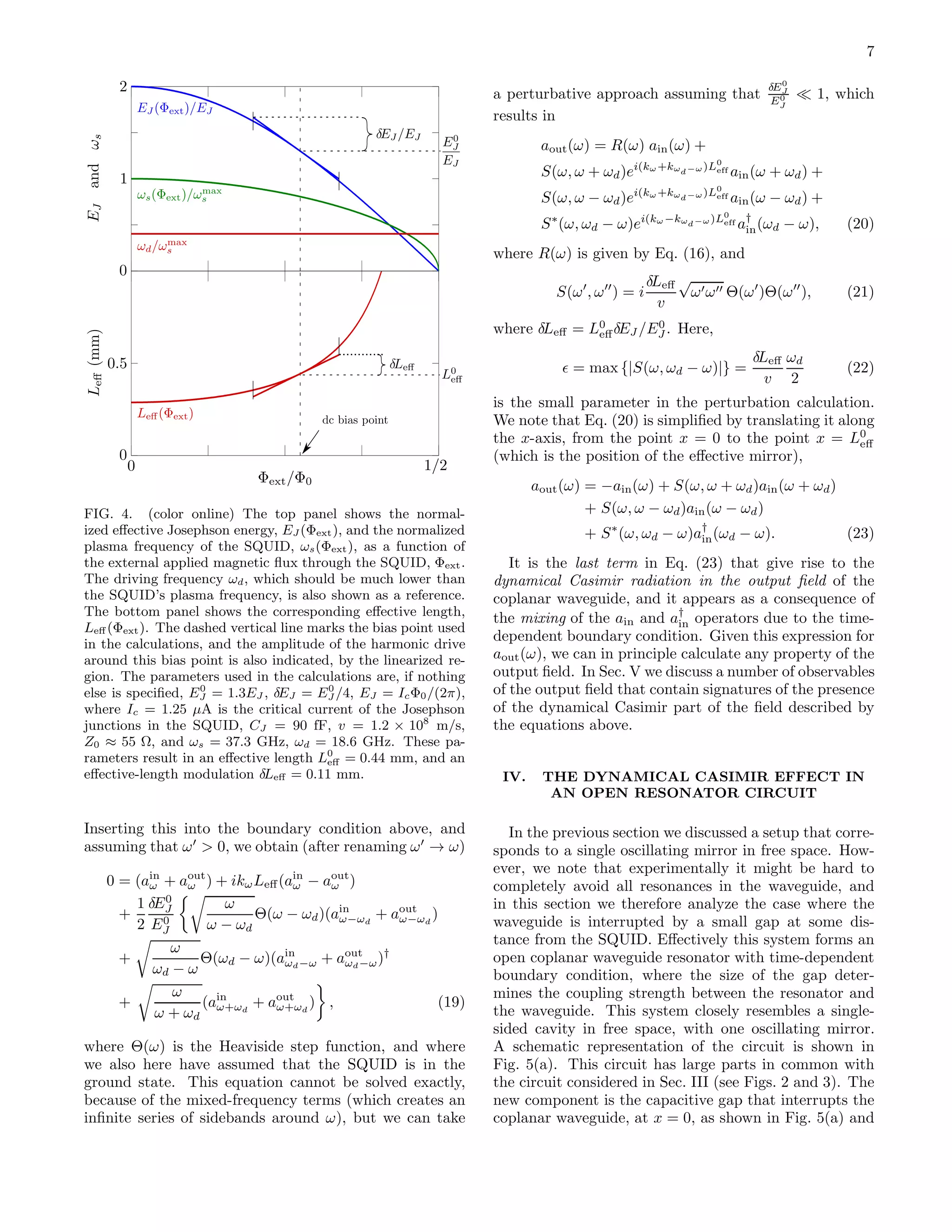
FIG. 2. (color online) (a) Schematic illustration of a copla-
nar waveguide terminated by a SQUID. The SQUID imposes
a boundary condition in the coplanar waveguide that can be
parametrically tuned by changing the externally applied mag-
netic flux through the SQUID. (b) The setup in (a) is equiv-
alent to a waveguide with tunable length, or to a mirror with
tunable position.
A. Quantum network analysis of the
SQUID-terminated coplanar waveguide
In this section we present a circuit model for the pro-
posed device and we derive the boundary condition of the
coplanar waveguide that is imposed by the SQUID (see
Fig. 2). The resulting boundary condition is then used in
the input-output formalism to solve for the output field
state, in the two cases of static and harmonic driving
of the SQUID. The circuit diagram for the device under
consideration is shown in Fig. 3, and the corresponding
circuit Lagrangian is
L =
1
2
∞
i=1
∆x C0( ˙Φi)2
−
(Φi+1 − Φi)2
∆xL0
+
j=1,2
CJ,j
2
( ˙ΦJ,j)2
+ EJ,j cos 2π
ΦJ,j
Φ0
, (4)
where L0 and C0 are, respectively, the characteristic in-
ductance and capacitance of the coplanar waveguide (per
unit length), and CJ,j and EJ,j are the capacitance and
Josephson energy of the jth junction in the SQUID loop.
Here, Φα is the node flux, which is related to the phase
ϕα, at the node α, as Φα = (Φ0/2π)ϕα, where Φ0 = h/2e
is the magnetic flux quantum.
We have assumed that the geometric size of the
SQUID loop is small enough such that the SQUID’s
self-inductance, Ls, is negligible compared to the ki-
netic inductance associated with the Josephson junctions

5. 5
...
...
FIG. 3. Equivalent circuit diagram for a coplanar waveguide
terminated by a SQUID. The coplanar waveguide has a char-
acteristic inductance L0 and capacitance C0, per unit length,
and it is assumed that it does not have any intrinsic dissipa-
tion. The circuit is characterized by the dynamical fluxes Φi
and ΦJ,j .
(Φ0/2π)2
/EJ,j (i.e., a term of the form LsI2
s has been
dropped from the Lagrangian above, where Is is the cir-
culating current in the SQUID). Under these conditions,
the fluxes of the Josephson junctions are related to the ex-
ternally applied magnetic flux through the SQUID, Φext,
according to ΦJ,1 − ΦJ,2 = Φext. We can therefore re-
duce the number of fluxes used to describe the SQUID
by introducing ΦJ = (ΦJ,1 + ΦJ,2)/2, and the SQUID
effectively behaves as a single Josephson junction [69].
Under the additional assumption that the SQUID is
symmetric, i.e., CJ,1 = CJ,2 = CJ /2 and EJ,1 = EJ,2 =
EJ , the Lagrangian now takes the form
L =
1
2
∞
i=1
∆x C0( ˙Φi)2
−
(Φi+1 − Φi)2
∆xL0
+
1
2
CJ ( ˙ΦJ )2
+ EJ (Φext) cos 2π
ΦJ
Φ0
, (5)
with effective junction capacitance CJ and tunable
Josephson energy
EJ (Φext) = 2EJ cos π
Φext
Φ0
. (6)
For a discussion of the case with asymmetries in the
SQUID parameters, see Ref. [11].
So far, no assumptions have been made on the cir-
cuit parameters that determine the characteristic energy
scales of the circuit, and both the waveguide fluxes and
the SQUID flux are dynamical variables. However, from
now on we assume that the plasma frequency of the
SQUID far exceeds other characteristic frequencies in the
circuit (e.g., the typical frequencies of the electromag-
netic fields in the coplanar waveguide), so that oscilla-
tions in the phase across the SQUID have small ampli-
tude, ΦJ /Φ0 ≪ 1, and the SQUID is operated in the
phase regime, where EJ (Φext) ≫ (2e)2
/2CJ . The condi-
tion ΦJ /Φ0 ≪ 1 allows us to expand the cosine function
in the SQUID Lagrangian, resulting in a quadratic La-
grangian
L =
1
2
∞
i=1
∆x C0( ˙Φi)2
−
(Φi+1 − Φi)2
∆xL0
+
1
2
CJ
˙Φ2
J −
1
2
2π
Φ0
2
EJ (Φext) Φ2
J . (7)
Following the standard canonical quantization proce-
dure, we can now transform the Lagrangian into a Hamil-
tonian which provides the quantum mechanical descrip-
tion of the circuit, using the Legendre transformation
H = i
∂L
∂ ˙Φi
˙Φi − L. We obtain the following circuit
Hamiltonian:
H =
1
2
∞
i=1
P2
i
∆xC0
+
(Φi+1 − Φi)2
∆xL0
+
1
2
P2
1
CJ
+
1
2
2π
Φ0
2
EJ (Φext) Φ2
1, (8)
and the commutation relations [Φi, Pj] = i¯hδij and
[Φi, Φj] = [Pi, Pj] = 0, where Pj = ∂L
∂ ˙Φj
. In the expres-
sion above we have also made the identification ΦJ ≡ Φ1
(see Fig. 3). The Heisenberg equation of motion for the
flux operator Φ1 plays the role of a boundary condition
for the field in the coplanar waveguide. By using the com-
mutation relations given above, the equation of motion
is found to be
˙P1 = CJ
¨Φ1 = −i[P1, H] =
= − EJ (Φext)
2π
Φ0
2
Φ1 −
1
L0
(Φ2 − Φ1)
∆x
, (9)
which in the continuum limit ∆x → 0 results in the
boundary condition [68]
CJ
¨Φ(0, t) +
2π
Φ0
2
EJ (t) Φ(0, t)
+
1
L0
∂Φ(x, t)
∂x x=0
= 0, (10)
where Φ1(t) ≡ Φ(x = 0, t), and EJ (t) = EJ [Φext(t)].
This is the parametric boundary condition that can be
tuned by the externally applied magnetic flux. Below
we show how, under certain conditions, this boundary
condition can be analogous to the boundary condition
imposed by a perfect mirror at an effective length from
the waveguide-SQUID boundary.
In a similar manner, we can derive the equation of
motion for the dynamical fluxes in the coplanar waveg-
uide (away from the boundary), i.e., for Φi, i > 1, which
results in the well-known massless scalar Klein-Gordon
equation. The general solution to this one-dimensional
wave equation has independent components that prop-
agate in opposite directions, and we identify these two
components as the input and output components of the
field in the coplanar waveguide.

6. 6
B. Quantization of the field in the waveguide
Following e.g. Refs. [66, 67], we now introduce creation
and annihilation operators for the flux field in the copla-
nar waveguide, and write the field in second quantized
form:
Φ(x, t) =
¯hZ0
4π
∞
0
dω
√
ω
ain(ω) e−i(−kωx+ωt)
+ aout(ω) e−i(kωx+ωt)
+ H.c. , (11)
where Z0 = L0/C0 is the characteristic impedance.
We have separated the left- and right-propagating sig-
nals along the x-axis, and denoted them as “output”
and “input”, respectively. The annihilation and cre-
ation operators satisfy the canonical commutation rela-
tion, [ain(out)(ω′
), a†
in(out)(ω′′
)] = δ(ω′
−ω′′
), and the wave
vector is defined as kω = |ω|/v, where v = 1/
√
C0L0 is
the propagation velocity of photons in the waveguide.
Our goal is to characterize the output field, e.g., by
calculating the expectation values and correlation func-
tions of various combinations of output-field operators.
To achieve this goal, we use the input-output formalism:
We substitute the expression for the field into the bound-
ary condition imposed by the SQUID, and we solve for
the output-field operators in terms of the input-field op-
erators. The input field is assumed to be in a known
state, e.g., a thermal state or the vacuum state.
C. Output field operators
By substituting Eq. (11) into the boundary condition,
Eq. (10), and Fourier transforming the result, we obtain
a boundary condition in terms of the creation and anni-
hilation operators (for ω′
> 0),
0 =
2π
Φ0
2 ∞
−∞
dω g(ω, ω′
) ×
Θ(ω)(ain
ω + aout
ω ) + Θ(−ω)(ain
−ω + aout
−ω)†
− ω′2
CJ (ain
ω′ + aout
ω′ ) + i
kω′
L0
(ain
ω′ − aout
ω′ ). (12)
where
g(ω, ω′
) =
1
2π
|ω′|
|ω|
∞
−∞
dt EJ (t)e−i(ω−ω′
)t
. (13)
This equation cannot be solved easily in general, but be-
low we consider two cases where we can solve it ana-
lytically, i.e., when EJ (t) is (i) constant, or (ii) has an
harmonic time-dependence. In the general case, we can
only solve the equation numerically, see Appendix A. In
Sec. V we compare the analytical results with such nu-
merical calculations.
1. Static applied magnetic flux
If the applied magnetic flux is time-independent,
EJ (t) = E0
J , we obtain g(ω, ω′
) = E0
J
ω′
ω δ(ω − ω′
),
and the solution takes the form
aout(ω) = R(ω) ain(ω), (14)
where
R(ω) = −
2π
Φ0
2
E0
J − |ω|2
CJ + ikω
L0
2π
Φ0
2
E0
J − |ω|2CJ − ikω
L0
. (15)
Assuming that the |ω|2
CJ term is small compared to
the other terms, i.e., that the SQUID plasma frequency
is sufficiently large, we can neglect it in the expression
above, and we are left with the following simplified form:
R(ω) = −
1 + ikωL0
eff
1 − ikωL0
eff
≈ − exp 2ikωL0
eff . (16)
Here, we have defined
L0
eff =
Φ0
2π
2
1
E0
J L0
, (17)
and assumed that kωL0
eff ≪ 1 (this condition gives an
upper bound on the frequencies for which this treatment
is valid). Figure 4 shows the dependences of EJ and Leff
on the externally applied magnetic flux Φext.
The reflection coefficient R(ω) on the simplified form
given above [Eq. (16)], exactly coincides with the reflec-
tion coefficient, − exp{2ikωL}, of a short-circuited copla-
nar waveguide of length L. It is therefore natural to inter-
pret the parameter L0
eff as an effective length that gives
the distance from the SQUID to a perfectly reflecting
mirror (which is equivalent to a short-circuit termination
in the context of coplanar waveguides). Alternatively,
this can be phrased in terms of boundary conditions,
where the mixed-type boundary condition Eq. (10) at
x = 0 is then equivalent to a Dirichlet boundary condi-
tion of an ideal mirror at x = L0
eff, for the frequencies
satisfying ω ≪ v/L0
eff. See, e.g., Refs. [60, 61] for dis-
cussions of different types of boundary conditions in the
context of the dynamical Casimir effect.
2. Weak harmonic drive
For a weak harmonic applied magnetic flux with fre-
quency ωd, giving EJ (t) = E0
J + δEJ cos(ωdt), with
δEJ ≪ E0
J , we obtain
g(ω, ω′
) = E0
J
|ω′|
|ω|
δ(ω − ω′
)
+ δE0
J
|ω′|
|ω|
1
2
[δ(ω − ω′
+ ωd) + δ(ω − ω′
− ωd)].
(18)

7. 7
FIG. 4. (color online) The top panel shows the normal-
ized effective Josephson energy, EJ (Φext), and the normalized
plasma frequency of the SQUID, ωs(Φext), as a function of
the external applied magnetic flux through the SQUID, Φext.
The driving frequency ωd, which should be much lower than
the SQUID’s plasma frequency, is also shown as a reference.
The bottom panel shows the corresponding effective length,
Leff (Φext). The dashed vertical line marks the bias point used
in the calculations, and the amplitude of the harmonic drive
around this bias point is also indicated, by the linearized re-
gion. The parameters used in the calculations are, if nothing
else is specified, E0
J = 1.3EJ , δEJ = E0
J /4, EJ = IcΦ0/(2π),
where Ic = 1.25 µA is the critical current of the Josephson
junctions in the SQUID, CJ = 90 fF, v = 1.2 × 108
m/s,
Z0 ≈ 55 Ω, and ωs = 37.3 GHz, ωd = 18.6 GHz. These pa-
rameters result in an effective length L0
eff = 0.44 mm, and an
effective-length modulation δLeff = 0.11 mm.
Inserting this into the boundary condition above, and
assuming that ω′
> 0, we obtain (after renaming ω′
→ ω)
0 = (ain
ω + aout
ω ) + ikωLeff(ain
ω − aout
ω )
+
1
2
δE0
J
E0
J
ω
ω − ωd
Θ(ω − ωd)(ain
ω−ωd
+ aout
ω−ωd
)
+
ω
ωd − ω
Θ(ωd − ω)(ain
ωd−ω + aout
ωd−ω)†
+
ω
ω + ωd
(ain
ω+ωd
+ aout
ω+ωd
) , (19)
where Θ(ω) is the Heaviside step function, and where
we also here have assumed that the SQUID is in the
ground state. This equation cannot be solved exactly,
because of the mixed-frequency terms (which creates an
infinite series of sidebands around ω), but we can take
a perturbative approach assuming that
δE0
J
E0
J
≪ 1, which
results in
aout(ω) = R(ω) ain(ω) +
S(ω, ω + ωd)ei(kω+kωd−ω)L0
eff ain(ω + ωd) +
S(ω, ω − ωd)ei(kω+kωd−ω)L0
eff ain(ω − ωd) +
S∗
(ω, ωd − ω)ei(kω−kωd−ω)L0
eff a†
in(ωd − ω), (20)
where R(ω) is given by Eq. (16), and
S(ω′
, ω′′
) = i
δLeff
v
√
ω′ω′′ Θ(ω′
)Θ(ω′′
), (21)
where δLeff = L0
effδEJ /E0
J . Here,
ǫ = max {|S(ω, ωd − ω)|} =
δLeff
v
ωd
2
(22)
is the small parameter in the perturbation calculation.
We note that Eq. (20) is simplified by translating it along
the x-axis, from the point x = 0 to the point x = L0
eff
(which is the position of the effective mirror),
aout(ω) = −ain(ω) + S(ω, ω + ωd)ain(ω + ωd)
+ S(ω, ω − ωd)ain(ω − ωd)
+ S∗
(ω, ωd − ω)a†
in(ωd − ω). (23)
It is the last term in Eq. (23) that give rise to the
dynamical Casimir radiation in the output field of the
coplanar waveguide, and it appears as a consequence of
the mixing of the ain and a†
in operators due to the time-
dependent boundary condition. Given this expression for
aout(ω), we can in principle calculate any property of the
output field. In Sec. V we discuss a number of observables
of the output field that contain signatures of the presence
of the dynamical Casimir part of the field described by
the equations above.
IV. THE DYNAMICAL CASIMIR EFFECT IN
AN OPEN RESONATOR CIRCUIT
In the previous section we discussed a setup that corre-
sponds to a single oscillating mirror in free space. How-
ever, we note that experimentally it might be hard to
completely avoid all resonances in the waveguide, and
in this section we therefore analyze the case where the
waveguide is interrupted by a small gap at some dis-
tance from the SQUID. Effectively this system forms an
open coplanar waveguide resonator with time-dependent
boundary condition, where the size of the gap deter-
mines the coupling strength between the resonator and
the waveguide. This system closely resembles a single-
sided cavity in free space, with one oscillating mirror.
A schematic representation of the circuit is shown in
Fig. 5(a). This circuit has large parts in common with
the circuit considered in Sec. III (see Figs. 2 and 3). The
new component is the capacitive gap that interrupts the
coplanar waveguide, at x = 0, as shown in Fig. 5(a) and

8. 8
(b). This gap is responsible for the formation of a res-
onator between the SQUID and the semi-infinite waveg-
uide, at x < 0. The coupling strength between the res-
onator and waveguide determines the quality factor of
the resonator. This quality factor, and the correspond-
ing decay rate, are important parameters in the following
analysis. Note that in the limit of vanishing quality fac-
tor this setup reduces to the setup studied in the previous
section.
Figure 5(b) shows a lumped circuit model for the part
of the circuit in the proximity of the capacitive gap. The
Lagrangian for this part of the circuit is
L =
1
2
∆xC0( ˙ΦL
0 )2
−
1
2
(ΦL
1 − ΦL
0 )2
∆x L0
+
1
2
∆xC0( ˙ΦL
1 )2
+ ...
+
1
2
∆xC0( ˙ΦR
0 )2
−
1
2
(ΦR
1 − ΦR
0 )2
∆x L0
+
1
2
∆xC0( ˙ΦR
1 )2
+ ...
+
1
2
Cc( ˙ΦL
0 − ˙ΦR
0 )2
, (24)
where ΦL
i and ΦR
i are the flux fields to the left and right of
the capacitive gap, respectively. In the continuum limit,
where ∆x → 0, the equations of motion for ΦL
0 and ΦR
0
result in the following boundary condition for the field in
the coplanar waveguide on both sides of the gap:
−
1
L0
∂ΦL
(x, t)
∂x x=0−
=Cc
∂2
ΦL
∂t2
x=0−
−
∂2
ΦR
∂t2
x=0+
1
L0
∂ΦR
(x, t)
∂x x=0+
=Cc
∂2
ΦR
∂t2
x=0+
−
∂2
ΦL
∂t2
x=0−
.
(25)
Using the field quantization from Sec. III, and Fourier
transforming the boundary condition above, results in a
boundary condition in terms of creation and annihilation
operators, in the frequency domain:
−
ikω
L0
aL
in(ω) − aL
out(ω) =
− ω2
Cc aL
in(ω) + aL
out(ω) − aR
in(ω) − aR
out(ω) (26)
ikω
L0
aR
in(ω) − aR
out(ω) =
− ω2
Cc aR
in(ω) + aR
out(ω) − aL
in(ω) − aL
out(ω) (27)
This system of equations can be solved, and the oper-
ators for the resonator can be written in terms of the
operators of the semi-infinite coplanar waveguide
aR
in(ω)
aR
out(ω)
=
1 − iωc
2ω iωc
2ω
−iωc
2ω 1 + iωc
2ω
aL
in(ω)
aL
out(ω)
, (28)
where ωc = (CcZ0)−1
is a parameter that characterizes
the coupling strength between the resonator and the open
coplanar waveguide. This transformation can be used to-
gether with Eq. (23), which relates the input and output
operators of the field in direct contact with the effective
mirror (i.e., aR
in(ω, x = deff) and aR
out(ω, x = deff), in the
present setup), to obtain a relation between aL
in(ω) and
FIG. 5. (color online) (a) Schematic drawing of a coplanar
waveguide (CPW) resonator, of length d, capacitively coupled
to an open, semi-infinite coplanar waveguide to the left, and
terminated to ground through a SQUID to the right. (b)
A magnification of the capacitive gap between the resonator
and the semi-infinite waveguide, shown as a dashed box in
(a), together with its equivalent circuit model.
aL
out(ω) that do not contain the resonator operators. To
achieve this we note that the resonator operators at x = 0
are related to those at x = deff by a simple phase factor,
according to the transformation
aR
in(ω, 0)
aR
out(ω, 0)
=
eikωdeff
0
0 e−ikωdeff
aR
in(ω, deff)
aR
out(ω, deff)
, (29)
and that aR
out(ω, 0) and aR
in(ω, 0) are related to aL
out(ω)
and aL
in(ω) according to the transformation in Eq. (28).
A. Output field operators
1. Static magnetic flux
The resonator boundary condition on the side that is
terminated by the SQUID is described by Eq. (23). In the
case of a static applied magnetic field the inelastic scat-
tering by the effective mirror is absent, i.e., S(ω′
, ω′′
) = 0,
and only the elastic reflections remain,
aR
out(ω, deff) = − aR
in(ω, deff). (30)
In the present setup, the SQUID is located at x = d,
and the effective mirror is located at x = deff, where
deff = d + L0
eff. Thus, to write a relation between the
input and output operator that applies on the left side
of the resonator, we translate the boundary condition of
the effective mirror by deff, according to Eq. (29),
aR
out(ω, 0) exp{−ikωdeff} = −aR
in(ω, 0) exp{ikωdeff}.(31)

9. 9
Since this relation applies at the point where the res-
onator is capacitively coupled to the open coplanar
waveguide, we can transform it using Eq. (28),
−i
ωc
2ω
aL
in(ω) + 1 + i
ωc
2ω
aL
out(ω) exp{−2ikωdeff}
= − 1 − i
ωc
2ω
aL
in(ω) + i
ωc
2ω
aL,0
out(ω) . (32)
This equation can be rewritten as
aL
out(ω) = Rres(ω)aL
in(ω), (33)
where
Rres(ω) =
1 + (1 + 2iω/ωc) exp{2ikωdeff}
(1 − 2iω/ωc) + exp{2ikωdeff}
. (34)
Similarly, we can apply Eq. (28) to solve for the res-
onator operators in terms of the input operators for the
coplanar waveguide,
aR
out(ω, deff) = Ares(ω)aL
in(ω), (35)
where
Ares(ω) =
(2iω/ωc) exp{ikωdeff}
(1 − 2iω/ωc) + exp{2ikωdeff}
, (36)
The function Ares(ω) describes the resonator’s response
to an input signal from the coplanar waveguide, and it
contains information about the mode structure of the
resonator. From Ares(ω) we can extract the resonance
frequencies and the quality factors for each mode, see
Fig. 6.
The resonance frequencies, ωres
n , are approximately
given by the transcendental equation
tan (2πωres
n /ω0) = ωc/ωres
n , (37)
where ω0 = 2πv/deff and n is the mode number. The
corresponding resonance widths and quality factors are
Γn = 2
ω0
2π
ωres
n
ωc
2
, (38)
Qn ≡
ωres
n
Γn
= 2π
ω2
c
2ω0ωres
n
, (39)
respectively. We note that the quality factor for higher-
order modes are rapidly decreasing as a function of the
mode number n (see also Fig. 6).
Using the expressions for ωres
n and Γn given above,
the resonator response can be expanded around the res-
onance frequencies and written in the form
Ares(ω) ≈ −
ω0
2π
Γn/2
Γn/2 − i(ω − ωres
n )
, (40)
and, similarly, the expression for the reflection coefficient
of the resonator from the open coplanar waveguide is
Rres(ω) ≈ −
Γn/2 + i(ω − ωres
n )
Γn/2 − i(ω − ωres
n )
. (41)
0
10
20
0 1 2
FIG. 6. (color online) The absolute value of Ares(ω) as a func-
tion of the renomalized frequency ω/ω0, where ω0 = 2πv/deff
is the full-wavelength resonance frequency when the resonator
is decoupled from the open coplanar waveguide. The sequence
of curves correspond to different coupling strengths to the
CPW, characterized by resonator ωc values indicated by the
labels in the figure.
2. Weak harmonic drive
For a time-dependent applied magnetic flux in the form
of a weak harmonic drive, we again take a perturbative
approach and solve the equations for aL
out(ω) in terms of
aL
in(ω) by treating S(ω′
, ω′′
) as a small parameter. Fol-
lowing the approach of the previous Section, we eliminate
the resonator variables by using Eq. (23) and Eq. (28),
and we obtain
aL
out(ω) = Rres(ω) aL
in(ω)
+ Sres,1(ω, ω + ωd)aL
in(ω + ωd)
+ Sres,1(ω, ω − ωd)aL
in(ω − ωd)
+ S∗
res,2(ω, ωd − ω)(aL
in)†
(ωd − ω), (42)
where Rres(ω) is given by Eq. (34), and
Sres,1(ω′
, ω′′
) = S(ω′
, ω′′
)Ares(ω′
)Ares(ω′′
), (43)
Sres,2(ω′
, ω′′
) = S(ω′
, ω′′
)A∗
res(ω′
)Ares(ω′′
). (44)
In this case the small parameter in the perturbation cal-
culation is
ǫres = max {|Sres,2(ω, ωd − ω)|} =
δLeff
deff
ωd
2
1
Γn
. (45)
We note that Eq. (42) has the same general form as
Eq. (23), and that the only differences are the defini-
tions of the reflection and inelastic scattering functions:
Rres(ω) and Sres,α(ω′
, ω′′
). This similarity allows us to

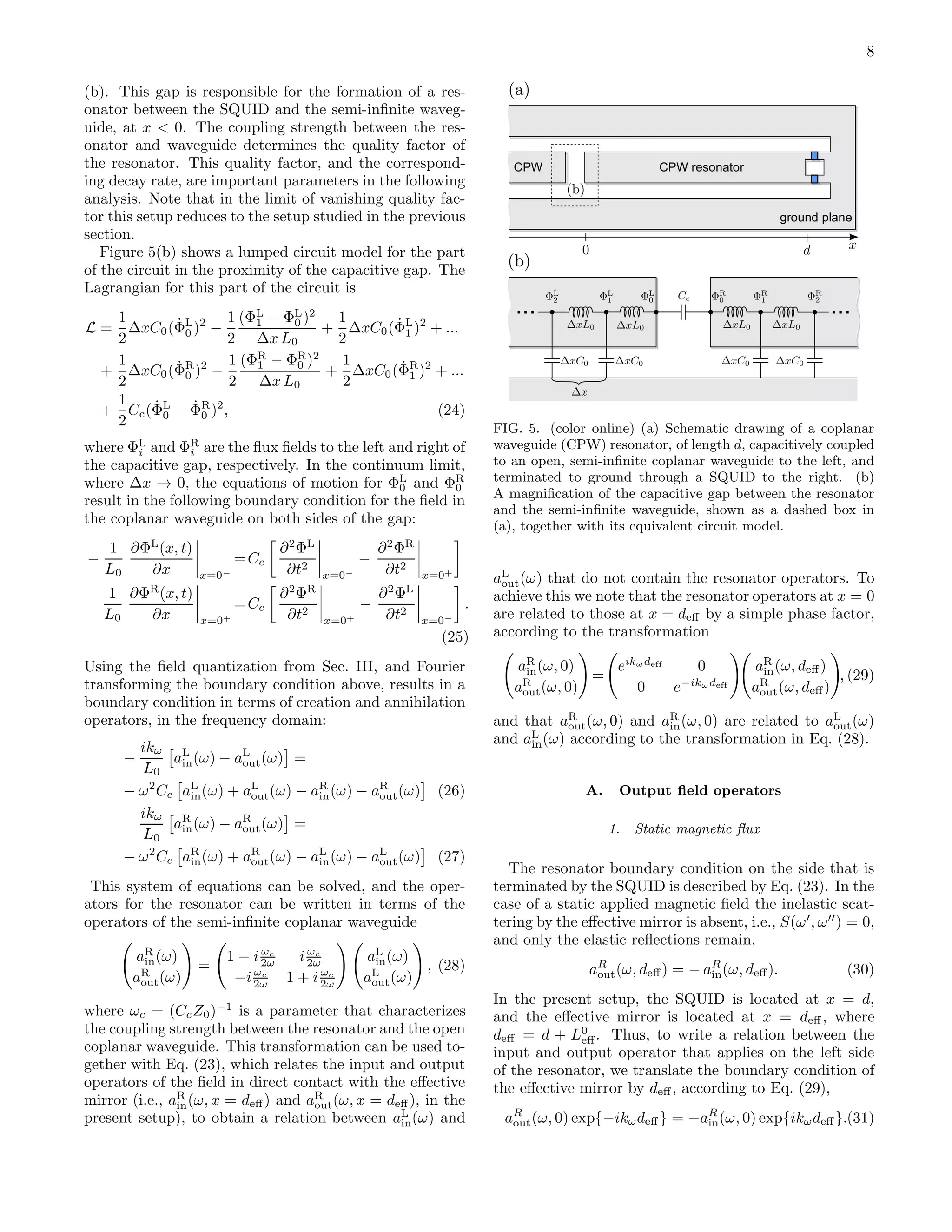
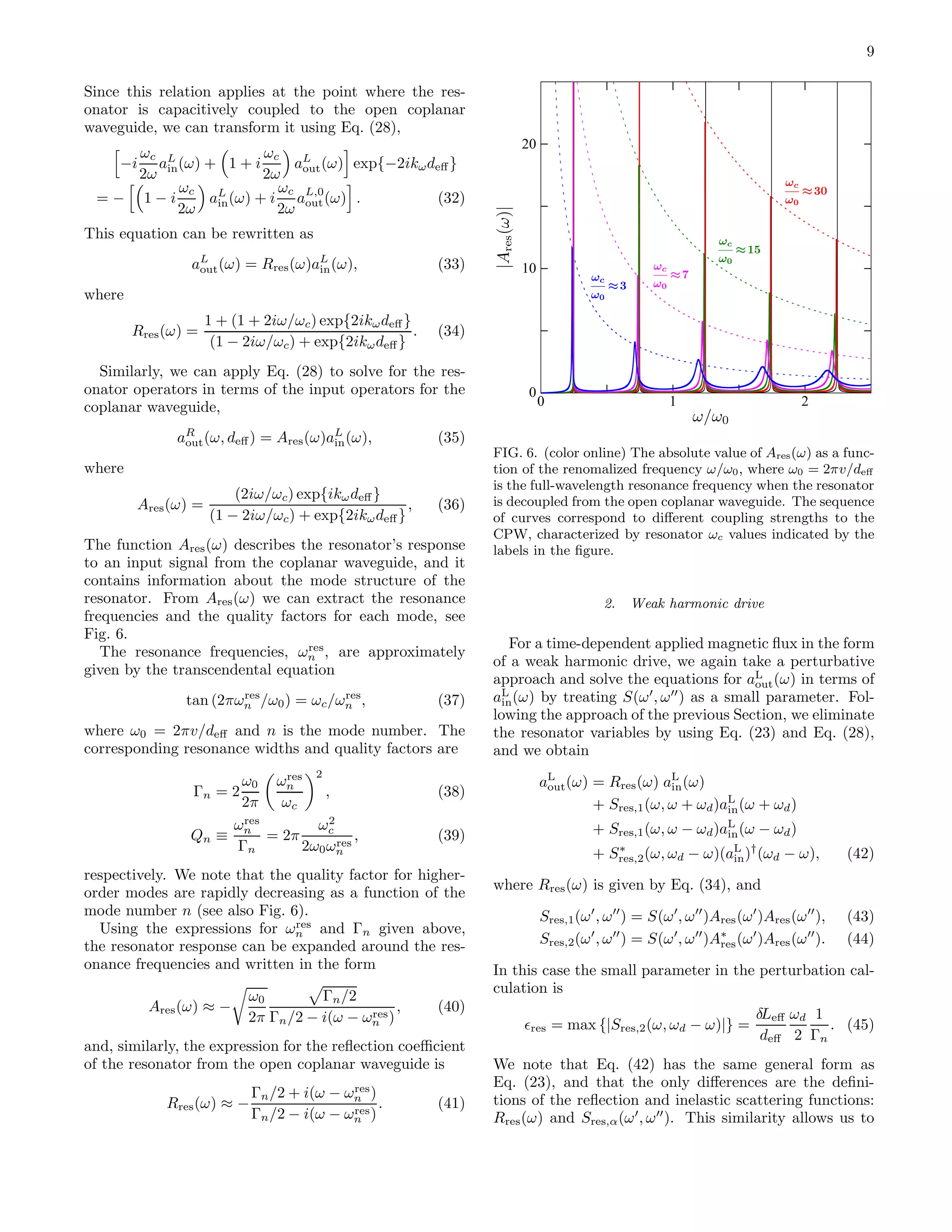
10. 10
CPW Resonator
SQUIDin
out
CPW
SQUIDin
out
Resonator circuit
Single-mirror circuit
FIG. 7. Schematic diagrams of the measurement setups for
(a) the single-mirror and (b) the resonator setups in super-
conducting microwave circuits, as discussed in Sec. III and
Sec. IV, respectively. The circulator (indicated by a circle
with a curved arrow) separates the input and output fields
such that only the signal from the SQUID reaches the mea-
surement device M, and so that the input-field state is given
by the thermal Johnson-Nyquist noise from the resistive load
R, at temperature T .
analyze both cases using the same formalism in the fol-
lowing sections, where we calculate expectation values
and correlation functions of physically relevant combina-
tions of the output field operators.
V. MEASUREMENT SETUPS
Equation (23) in Sec. III, and Eq. (42) in Sec. IV,
constitute complete theoretical descriptions of the cor-
responding output fields, and we can apply these expres-
sions in calculating the expectation values of any output-
field observable or correlation function. In this Section we
discuss possible experimental setups for measuring vari-
ous physical properties of the output field, and we discuss
which quantum mechanical observables and correlation
functions these setups measure, in terms of the output-
field operators. Below, we use Eq. (23) and Eq. (42), and
explicitly evaluate these physical observables for the two
setups discussed in the previous Sections.
The basic setups that we are considering here are
shown schematically in Fig. 7, which also illustrates the
concept of separating the incoming and the outgoing
fields by means of a circulator. The input field is ter-
minated to ground through an impedance-matched re-
sistive load. This resistor produces a Johnson-Nyquist
(thermal) noise that acts as the input on the SQUID.
The circulator isolates the detector from the thermal sig-
nal from the resistor, except for the part of the noise
that is reflected on the SQUID. The measurement device
is denoted by M in these circuits.
We are interested in experimentally relevant observ-
ables that contain signatures of the dynamical Casimir
part of the output field, i.e., the part that is described
by the fourth term in Eq. (23) and Eq. (42). The most
signal
signal
Intensity correlation measurement setup
Quadrature squeezing measurement setup
FIG. 8. Schematic measurement setups for (a) intensity corre-
lations and for (b) quadrature squeezing. In (a), the box with
τ inside represents a time-delay, and in (b) the box with the
label LO represents a local oscillator. The microwave beam
splitter can be implemented, e.g., by a hybrid ring. The de-
tectors are assumed to measure the intensity of the voltage
field. In a practical experimental setup, the signals would also
have to pass through several stages of amplification, which are
not shown here.
distinct signature of the dynamical Casimir effect is per-
haps the correlations between individual pairs of photons,
and such correlations could in principle be measured in
a coincidence-count experiment. However, the physical
quantities that can be measured in a microwave circuit
are slightly different from those measured in the quantum
optics regime. For instance, there are currently no single-
photon detectors available in the microwave regime, and
as a consequence it is not possible to directly measure
the correlations between individual pairs of photons. In-
stead, there are linear amplifiers [75] that can amplify
weak signals, with very low-intensity photon-flux densi-
ties, to larger signals that can be further processed with
classical electronics. In addition to amplifying the signal,
these amplifiers also add noise [76, 77] to the signal. How-
ever, the increased noise can often be compensated for,
e.g., by averaging the signal over long a period of time, or
by measuring cross-correlations in which the noise mostly
cancel out.
In microwave electronics, the natural fields for describ-
ing the coplanar waveguides are the current and voltage
fields, and these physical quantities can be readily mea-
sured with standard equipment. Here we therefore focus
on the voltage V (x, t) in the coplanar waveguide as our
main physical observable. The voltage is related to the
previously defined field creation and annihilation opera-
tors according to
Vout(x, t) = ∂tΦout(x, t) =
¯hZ0
4π
∞
0
dω
√
ω −iaout
ω e−i(kωx+ωt)
+ H.c. . (46)
The output field states described by Eq. (23) and
Eq. (42) have voltage expectation values that are zero,
Vout(x, t) = 0, but the squared voltages, i.e., as mea-
sured by a voltage square-law detector, and various forms

11. 11
of voltage correlations, can have non-zero expectation
values. For example, Vout(x, t)2
, Vout(t1)Vout(t2) ,
and Vout(ω1)Vout(ω2) , are all in general non-zero, and
do contain signatures of the presence of the dynamical
Casimir radiation.
A. Photon-flux density
To measure the photon-flux density requires an inten-
sity detector, such as a photon counter that clicks each
time a photon is absorbed by the detector. The mea-
sured signal is proportional to the rate at which the de-
tector absorbs photons from the field, which in turn is
proportional to the field intensity. This detector model
is common in quantum optics, and it is also applicable to
intensity detectors (such as voltage square-law detectors)
in the microwave regime, although not with single-photon
resolution.
The signal recorded by a quantum mechanical pho-
ton intensity (power) detector (see, e.g., Ref. [74]) in the
coplanar waveguide corresponds to the observable
I(t) ∝ Tr ρ ˆV (−)
(x, t) ˆV (+)
(x, t) , (47)
where V (±)
(x, t) are the positive and negative frequency
component of the voltage field, respectively. In terms of
the creation and annihilation operators for the field in the
coplanar waveguide [see Eq. (46)], where we, for brevity,
have taken x = 0,
I(t) ∝
∞
0
dω′
∞
0
dω′′
√
ω′ω′′ Tr ρa†
ω′ aω′′ ei(ω′
−ω′′
)t
,
(48)
and the corresponding noise-power spectrum is
SV (ω) =
∞
0
dω′
Tr ρ ˆV (−)
(ω) ˆV (+)
(ω′
)
=
¯hZ0
4π
∞
0
dω′
√
ωω′ n(ω, ω′
), (49)
where n(ω, ω′
) = Tr ρa†
(ω)a(ω) . Here, SV (ω) is related
to the voltage auto-correlation function via a Fourier
transform, according to the Wiener-Khinchin theorem.
The photon-flux density in the output field,
nout(ω) =
∞
0
dω′
nout(ω, ω′
), (50)
can be straightforwardly evaluated using Eq. (23). The
resulting expression is
nout(ω) = |R(ω)|2
¯nin(ω) + |S(ω, ω + ωd)|2
¯nin(|ω + ωd|)
+ |S(ω, |ω − ωd|)|2
¯nin(|ω − ωd|)
+ |S(ω, ωd − ω)|2
Θ(ωd − ω), (51)
where ¯nin(ω) = Tr ρa†
in(ω)ain(ω) is the thermal pho-
ton occupation of the input-field mode with frequency
0
1
2
3
4
0 1 2
thermal only
analytical,
thermal & DCE
numerical,
thermal & DCE
FIG. 9. (color online) The output-field photon-flux density,
nout(ω), as a function of the relative mode frequency ω/ωd,
for the single-mirror setup. The solid and the dashed curves
are for the temperatures T = 50 mK and T = 25 mK, re-
spectively, and the dotted curve is for zero temperature. The
red (bottom) curves show the part of the signal with ther-
mal origin, and the blue (dark) and the green (light) curves
also include the radiation due to the dynamical Casimir ef-
fect. The blue curves are the analytical results, and the green
curves are calculated numerically using the method described
in Appendix A. The parameters are the same as in Fig. 4.
The presence of the dynamical Casimir radiation is clearly
distinguishable for temperatures up to ∼ 70 mK. The good
agreement between the analytical and numerical results veri-
fies the validity of the perturbative calculation for the param-
eters used here.
ω, given by ¯nin
ω = [exp(¯hω/kbT ) − 1]−1
, where T is the
temperature and kB is the Boltzmann constant.
The first three terms in the expression above are of
thermal origin, and the fourth term is due to the dynam-
ical Casimir effect. In order for the dynamical Casimir
effect not to be negligible compared to the thermally ex-
cited photons, we require that kbT ≪ ¯hωd, where the
driving frequency ωd here serves as a characteristic fre-
quency for the system, since all dynamical Casimir ra-
diation occurs below this frequency (to leading order).
In this case it is safe to neglect the term containing the
small factor ¯nin(|ω + ωd|) in the expression above. Sub-
stituting the expression for S(ω, ωd), from Eq. (21), into
Eq. (51), results in the following explicit expression for
the output field photon flux, for the single-mirror case:
nout(ω) = ¯nin(ω) +
δLeff
v
2
ω |ω − ωd| ¯nin(|ω − ωd|)
+
δLeff
v
2
ω(ωd − ω) Θ(ωd − ω).(52)

12. 12
0
2
4
6
8
0 10.5
resonance frequencies
FIG. 10. (color online) The output photon-flux density,
nout(ω), for the resonator setup (solid lines), as a function
of the normalized frequency ω/ωd, for four difference reso-
nance frequencies (marked by dashed vertical lines). Note
that a double-peak structure appears when the driving fre-
quency is detuned from twice the resonance frequency. For
reference, the result for the single-mirror setup is also shown
(red solid curve without resonances). Here, the temperature
was chosen to be T = 25 mK, and the quality factor of the
first resonance mode is Q0 ≈ 20 (ωc ≈ 3ωd), see Eq. (39).
The other parameters are the same as in Fig. 4.
The output-field photon flux density, Eq. (52), is plot-
ted in Fig. 9. The blue dotted parabolic contribution to
nout(ω) is due to the fourth term in Eq. (51), i.e., the
dynamical Casimir radiation [compare Eq. (2)].
Similarly, by using Eq. (42), we calculate the output-
field photon-flux density for the setup with a resonator,
and the resulting expression also takes the form of
Eq. (51), but where R(ω) and S(ω′
, ω′′
) are given by
Eq. (34) and Eq. (43), respectively. The resulting
photon-flux density for the resonator setup is plotted in
Fig. 10. Here, photon generation occurs predominately in
the resonant modes of the resonator. For significant dy-
namical Casimir radiation to be generated it is necessary
that the frequencies of both generated photons (ω′
and
ω′′
, where ω′
+ ω′′
= ωd) are near the resonant modes of
the resonator. In the special case when the first resonance
coincide with half of the driving frequency, ωres
n = ωd/2,
there is a resonantly-enhanced emission from the res-
onator, see Fig. 10. The resonant enhancement is due to
parametric amplification of the electric field in the res-
onator (i.e., amplification of both thermal photons and
photons generated from vacuum fluctuations due to the
dynamical Casimir effect).
Another possible resonance condition is
ωres
0 + ωres
1 ∼ ωd. (53)
In this case, strong emission can occur even when the
0
1
2
3
4
0 1 1.50.5
FIG. 11. (color online) The output photon-flux density,
nout(ω), as a function of normalized frequency, for the res-
onator setups where two modes (blue) and a single mode
(green) are active in the dynamical Casimir radiation. The
dashed and the dotted vertical lines mark the resonance fre-
quencies of the few lowest modes for the two cases, respec-
tively. The solid red curve shows the photon-flux density in
the absence of the resonator. The blue solid curve is the
photon-flux density for the two-mode resonance, i.e., for the
case when the two lowest resonance frequencies add up to
the driving frequency. The green curve shows the photon-flux
density for the case when only a single mode in the resonator
is active (see Fig. 10 for more examples of this case). Here,
the temperature was chosen to be T = 10 mK, and the res-
onator’s quality factor is in both cases Q0 ≈ 50. The other
parameters are the same as in Fig. 4.
frequencies of the two generated photons are significantly
different, since the two photons can be resonant with
different modes of the resonator, i.e., ω′
∼ ωres
0 and ω′′
∼
ωres
1 . See the blue curves in Fig. 11.
We conclude that in the case of a waveguide without
any resonances the observation of the parabolic shape of
the photon-flux density nout(ω) would be a clear signature
of the dynamical Casimir effect. The parabolic shape
of the photon-flux density should also be distinguishable
in the presence of a realistic thermal noise. Resonances
in the waveguide concentrate the photon-flux density to
the vicinity of the resonance frequencies, which can give
a larger signal with a smaller bandwidth. One should
note that in order to stay in the perturbative regime,
the driving amplitude should be reduced by the quality
factor of the resonance, compared to the case without
any resonances. The bimodal structure of the spectrum,
and its characteristic behavior as a function of the driving
frequency and detuning, should be a clear indication of
the dynamical Casimir effect.

13. 13
B. Two-photon correlations
The output fields described by Eq. (23) and Eq. (42)
exhibit correlations between photons at different frequen-
cies. This is straightforwardly demonstrated by calcu-
lating the expectation value of the photon-annihilation
operators at two frequencies symmetric around half the
driving frequency, i.e.,
aout
ωd
2
− ∆ω aout
ωd
2
+ ∆ω =
R
ωd
2
− ∆ω S∗ ωd
2
+ ∆ω,
ωd
2
− ∆ω ×
1 + ¯nin
ωd
2
− ∆ω , (54)
which can be interpreted as the correlation (entangle-
ment) between two photons that are simultaneously cre-
ated at the frequencies ωd/2−∆ω and ωd/2+∆ω, where
∆ω < ωd/2. This two-photon correlation is shown in
Fig. 12, for the field generated by the SQUID without
the resonator (shown in blue), and with the resonator
(shown in red). Note that for thermal and vacuum states
this expectation value vanishes for all frequencies ω. This
correlation is not directly measurable, since the operator
combination is not Hermitian, but it serves the purpose of
being the most basic illustration of the presence of non-
classical two-photon correlations in the field produced
by the dynamical Casimir effect. Below we consider two
physically observable correlation functions that are ex-
perimentally measurable.
1. Second-order coherence function
The fact that photons are predicted to be generated in
pairs in the dynamical Casimir effect implies that the
time-domain photon statistics exhibits photon bunch-
ing. For instance, the measurement setup outlined in
Fig. 8(a), which measures the second-order correlation
function
G(2)
(τ) = Tr ρV (−)
(0)V (−)
(τ)V (+)
(τ)V (+)
(0) , (55)
could be used to detect this bunching effect. For the
output fields on the form of Eqs. (23) and (42), this cor-
relation function takes the form
G(2)
(τ) = |G(1)
(τ)|2
+
ωd
0
dω ω |S(ω, ωd − ω)|2
eiωτ
2
+
ωd
0
dω ω(ωd − ω)R(ωd − ω)S∗
(ω, ωd − ω)eiωτ
2
,
G(1)
(τ) =
ωd
0
dω ω|S(ω, ωd − ω)|2
, (56)
where R(ω) and S(ω′
, ω′′
) are defined by Eqs. (15,21) and
(34,44) for the two setups, respectively. The normalized
second-order correlation function, i.e., the second-order
0
0.1
0 0.25 0.5
0.05 single mirror
with resonator
FIG. 12. (color online) Correlations between photons at the
frequencies ωd/2 − ∆ω and ωd/2 + ∆ω, as a function of de-
tuning ∆ω from half the driving frequency, for the single-
mirror setup (blue) and the setup with a resonator (red) that
is slightly detuned from half the driving frequency, ωd/2. The
dashed blue curve shows the correlations for single-mirror
setup in the presence of thermal noise, at T = 25 mK.
1
2
0 1 2 3 4 5
0
1
0 1 2 3 4 5
single mirror
with resonator
single mirror
FIG. 13. The normalized second-order coherence function,
g2(τ), as a function of the delay time τ, for the field pro-
duced by the single-mirror setup from Sec. III (in blue),
and for the resonator setup (in red), at zero temperature.
The inset shows the second-order coherence function for the
single-mirror setup without the normalization, illustrating
that g2(τ) > 1 and showing the oscillating behavior of g2(τ)
for large τ.
coherence function
g(2)
(τ) =
G(2)
(τ)
G(1)(0)G(1)(τ)
, (57)
is shown in Fig. 13 for the single-mirror setup (blue) and
the resonator setup (red). These coherence functions
show clear photon bunching, since g(2)
(τ) > 1 for a large

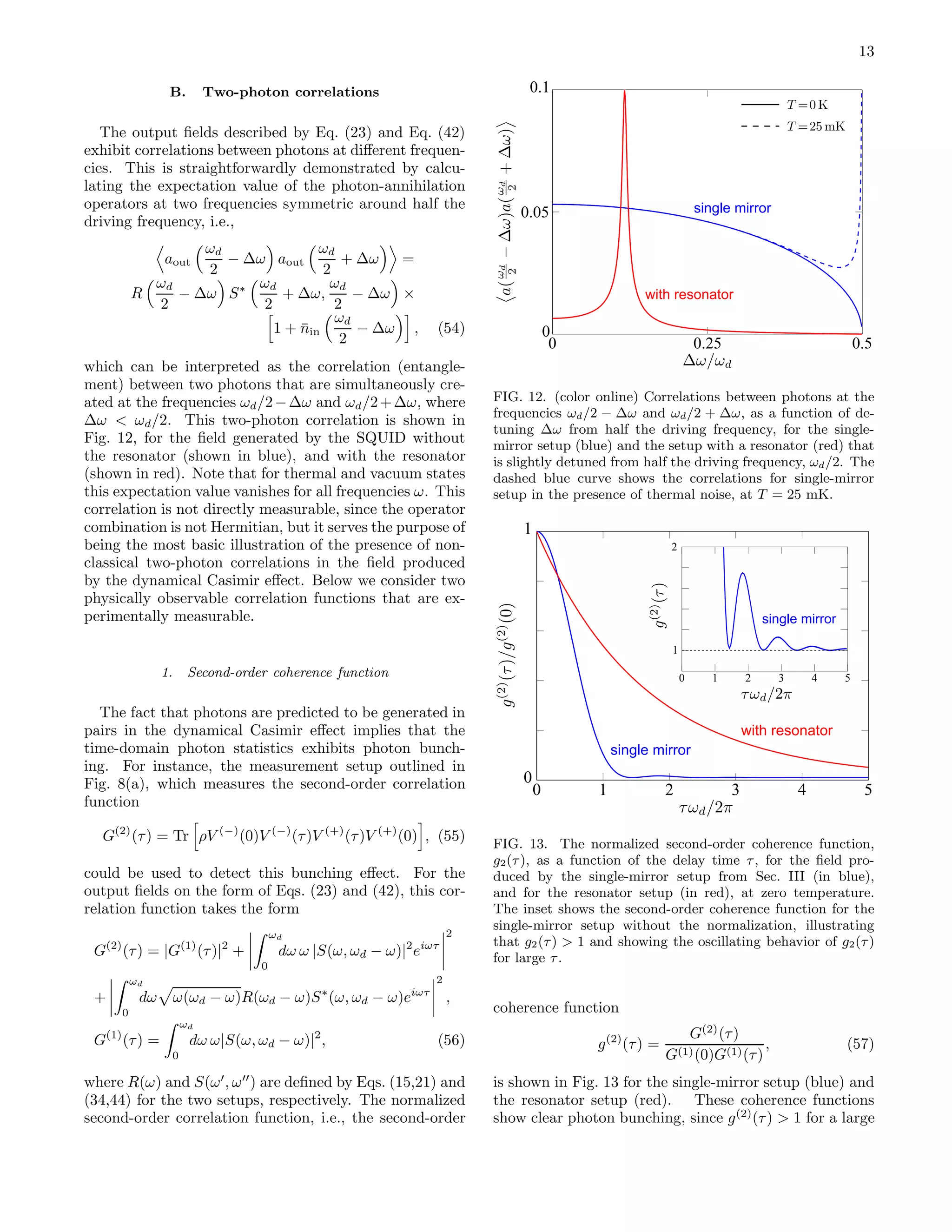
14. 14
range in τ. In particular, for zero time-delay, τ = 0, the
coherence functions can be written as
g(2)
(0) = 2 +
1
ǫ2
, (58)
where ǫ is given by Eq. (22) for the single-mirror setup,
and by Eq. (45) for the resonator setup, as discussed
in Sec. III and Sec. IV, respectively. In both cases, ǫ is
small and g(2)
(0) ≫ 1, which corresponds to large photon
bunching. The high value of g(2)
(0) can be understood
from the fact that the photons are created in pairs, so
the probability to detect two photons simultaneously is
basically the same as the probability to detect one pho-
ton. For low photon intensities, this gives a very large
second-order coherence. The decay of g(2)
(τ) is given by
the bandwidth of the photons, which in the case without
resonance is given by the driving frequency ωd. When
a resonance is present, its bandwidth Γ determines the
decay. Squeezed states show this type of photon bunch-
ing [70], and we now proceed to calculate the squeezing
spectrum of the radiation.
2. Squeezing spectrum
Another nonclassical manifestation of the pairwise
photon correlation in the fields described by Eqs. (23)
and (42) is quadrature squeezing [71, 72] and the corre-
sponding squeezing spectrum [73], defined as the quadra-
ture squeezing at a certain frequency. The quadratures
in the frequency domain are defined by the relation
Xθ(ω) =
1
2
a(ω)e−iθ
+ a†
(ω)eiθ
, (59)
so that X1 = Xθ=0, and X2 = Xθ=π/2. Experimen-
tally, the quadratures in a continuous multimode field
can be measured through homodyne detection, where the
signal field is mixed with a local oscillator (LO) on a
balanced beam splitter, resulting in aout(t) = (aLO(t) +
asig(t))/
√
2. See Fig. 8(b) for a schematic representa-
tion of this setup. The local oscillator field is assumed
to be in a large-amplitude coherent state with frequency
Ω and phase θ, i.e., aLO = |α| exp{−i(θ + Ωt)}. Probing
the resulting output field with an intensity detector then
provides information about the quadrature in the signal
field, since
I(t) = a†
out(t)aout(t) ≈ |α|2
+ |α| Xθ
out(t) (60)
where
Xθ
out(t) =
1
2
asig(t)ei(θ+Ωt)
+ a†
sig(t)e−i(θ+Ωt)
. (61)
The noise-power spectrum of the voltage intensity of the
output field therefore gives the squeezing spectrum of the
signal field, in the frame rotating with frequency Ω:
Sθ
X(∆ω) = 1+4
∞
−∞
dt e−i∆ωt
: ∆Xθ
out(t)∆Xθ
out(0) : ,
(62)
0.6
1.0
1.4
-0.5 -0.25 0 0.25 0.5
with resonator
without resonator
squeezing spectrum
for a parametric oscillator with
a Kerr nonlinearity
variances in
variances in
FIG. 14. (color online) The spectra of quadrature squeezing in
the output field for a SQUID-terminated coplanar waveguide
with (solid lines) and without (dashed lines) a resonator, as a
function of the renormalized frequency detuning from ωd/2.
The blue (dark) and the red (light) lines correspond to the
variances in the Xθ− and Xθ+ quadrature, respectively. For
reference, the dotted thin lines show the squeezing spectrum
for the field produced by a parametric oscillator with a Kerr
nonlinearity.
where : : is the normally-ordered expectation value,
and where we have normalized the squeezing spectrum
so that Sθ
X = 1 for unsqueezed vacuum, and Sθ
X = 0
corresponds to maximum squeezing. Here, ∆ω is the fre-
quency being measured after the mixing with the local
oscillator, and it is related to the frequency ω in the sig-
nal field as ω = Ω + ∆ω. Hereafter, we choose Ω = ωd
2 .
Evaluating the squeezing spectrum for the quadrature
defined by the relative phase θ, i.e., Xθ
out(t), results in
Sθ
X(∆ω) = 1 + 2 S
ωd
2
+ ∆ω,
ωd
2
− ∆ω
2
+ e−2iθ
R
ωd
2
+ ∆ω S
ωd
2
+ ∆ω,
ωd
2
− ∆ω
+ e2iθ
R∗ ωd
2
− ∆ω S∗ ωd
2
− ∆ω,
ωd
2
+ ∆ω (63)
where, as before, R(ω) and S(ω′
, ω′′
) are defined by
Eqs. (15,21) and Eqs. (34,43) for the two setups, respec-
tively.
For the single-mirror setup discussed in Sec. III, we
obtain the following squeezing spectrum
Sθ
X (∆ω) ≈ 1 − 2ǫ sin(2θ) 1 − 4
∆ω
ωd
2
, (64)
where we have neglected the second term in Eq. (63),
which is one order higher in the small parameter
S(ω′
, ω′′
). Here, we can identify the relative phases θ−
=

15. 15
π/4 and θ+
= −π/4 as the maximally-squeezed quadra-
ture (θ−
) and the corresponding orthogonal quadrature
(θ+
).
By using the expressions for reflection and inelastic
scattering of the resonator setup, Eqs. (34,43), in the ex-
pression for the squeezing spectrum, Eq. (63), we obtain
Sθ±
X (∆ω) ≈ 1 ±
2ǫres
1 + 2∆ω
Γ
2 , (65)
where the frequency of the first resonator mode is as-
sumed to coincide with half the driving frequency, ωres
0 =
ωd/2, and where we again have defined θ±
= ∓π/4 to
correspond to the maximally-squeezed quadrature and
the corresponding orthogonal quadrature. The squeez-
ing spectra for the single-mirror setup, Eq. (64), and for
the resonator setup, Eq. (65), are plotted in Fig. 14. The
squeezing is limited by ǫ and ǫres, respectively, and it is
therefore not possible to achieve perfect squeezing, but as
shown in Fig. 14, significant squeezing is still possible. In
the single-mirror case the squeezing covers a large band-
width, and the total squeezing (see, e.g., Ref. [73]) of the
Xθ− quadrature, given by the integral of SX (ω, θ−
), is
STotal
X (θ−
) ≈ ωd 1 −
π
2
ǫ . (66)
VI. COMPARISON WITH A PARAMETRIC
OSCILLATOR
As the Qn values of the resonator considered in Sec. IV
increases, its resonant modes are increasingly decoupled
from the coplanar waveguide, and the modes become in-
creasingly equidistant. In the limit Qn → ∞, the sys-
tem formally reduces to the ideal case of a closed one-
dimensional cavity (see, e.g., Refs. [1, 48–50]). However,
this limit is not realistic for the type of circuits inves-
tigated here, because it corresponds to a regime where
also the high-frequency modes are significantly excited,
and this would violate our assumption that the SQUID is
adiabatic (i.e., that the SQUID plasma frequency is the
largest frequency in the problem). Our theoretical anal-
ysis is also unsuitable for studying that extreme limit,
since it implies that ǫres no longer is small.
However, for moderate Q0-values, where ǫres is small
and our analysis applies, it is still possible to make a
comparison to a single-mode parametric oscillator (PO)
below its threshold. The Hamiltonian for a pumped
parametric oscillator [73] with a Kerr-nonlinearity can
be written as
HPO =
¯hω2
2
a†
a +
1
2
i¯h e−iωdt
ǫ a† 2
− eiωdt
ǫ∗
a2
,(67)
and where the oscillator is assumed to couple to an en-
vironment that induces relaxation with a rate γ. The
output field for the parametric oscillator is described by
aPO
out(ω) = F(ω)aPO
in (ω) + G(ω)aPO
in (−ω)†
, (68)
where
F(ω) =
(γ/2)
2
+ ω2
+ |ǫ|2
(γ/2 − iω)
2
− |ǫ|2
, (69)
G(ω) =
γǫ
(γ/2 − iω)
2
− |ǫ|2
, (70)
see, e.g., Ref. [73]. Comparing Eq. (68) to the corre-
sponding results for the dynamical Casimir effect:
aDCE
out (ω) = Rres
ωd
2
+ ω aDCE
in (ω)
+ S∗
res
ωd
2
− ω,
ωd
2
+ ω aDCE
in (−ω)†
, (71)
where Rres(ω) and Sres(ω′
, ω′′
) are given by Eqs. (34,44),
allows us to identify relations between the parametric os-
cillator parameters (to first order in ǫ) and the dynamical
Casimir parameters. We obtain
γ = Γ0, (72)
ǫ = −i
δLeff ωd
4 deff
, (73)
and thereby establish a one-to-one mapping between
these systems, valid for sufficiently large Q and below
the parametric oscillator threshold: ǫ < γ/2, i.e., for
δLeff
deff
ωd
2Γ
< 1. (74)
Using these expressions we can write a Hamiltonian that
describes the dynamical Casimir effect in the resonator
setup,
HDCE =
¯hωd
2
a†
a −
δLeff
4deff
¯hωd
2
eiωdt
a2
+ e−iωdt
a† 2
,
(75)
and where the capacitive coupling to the open coplanar
waveguide induces relaxation with a rate Γ0 in the res-
onator. This Hamiltonian picture offers an alternative
description of the photon creation process in the dynam-
ical Casimir effect in a resonator. This correspondence
between the dynamical Casimir effect and a parametric
oscillator was also discussed in e.g. Ref. [78].
VII. SUMMARY AND CONCLUSIONS
We have analyzed the dynamical Casimir radiation
in superconducting electrical circuits based on coplanar
waveguides with tunable boundary conditions, which are
realized by terminating the waveguides with SQUIDs.
We studied the case of a semi-infinite coplanar wave-
guide, and the case of a coplanar waveguide resonator
coupled to a semi-infinite waveguide, and we calculated
the photon flux, the second-order coherence functions
and the noise-power spectrum of field quadratures (i.e.,
the squeezing spectrum) for the radiation generated due
to the dynamical Casimir effect. These quantities have

16. 16
Single-mirror DCE Low-Q resonator DCE High-Q resonator DCE / PO
Comments
Photons created due to
time-dependent boundary
condition.
The resonator slightly alters
the mode density, compared to
the single-mirror case.
DCE in a high-Q resonator is
equivalent to a PO below
threshold.
Classical analogue? No, requires vacuum
fluctuations.
No, requires vacuum
fluctuations.
Yes, vacuum and thermal
fluctuations give similar
results.
Resonance condition no resonator ωres = ωd/2 ωres = ωd/2
Threshold condition – ǫres ∼ Q−1
ǫres ∼ Q−1
≪ 1
Above threshold: nonlinearity
dominates behavior.
Number of DCE
photons per second
∼ n(ωd/2) ωd ∼ n(ωres) Γ ∼ n(ωres) Γ
Spectrum
at T = 0 K
Broadband spectrum with
peak at ωd/2
on resonance off resonance
Broad peaks at resonance
frequency ωres and the
complementary frequency
ωd − ωres.
Sharply peaked around the
resonance frequency
ωres = ωd/2.
TABLE III. Comparison between the dynamical Casimir effect (DCE), in the single-mirror setup and the resonator setup, with
a parametric oscillator (PO) with a Kerr nonlinearity. In Sec. VI we showed that in the high-Q limit, the dynamical Casimir
effect in the resonator setup is equivalent to a parametric oscillator. In the very-high-Q limit, the dynamics involves many
modes of the resonator. We do not consider the latter case here.
distinct signatures which can be used to identify the dy-
namical Casimir radiation in experiments.
For the single-mirror setup, we conclude that the
photon-flux density nout(ω) has a distinct inverted
parabolic shape that would be a clear signature of the
dynamical Casimir effect. This feature in the photon-flux
density should also be distinguishable in the presence of
a realistic thermal noise background.
For the resonator setup, the presence of resonances
in the coplanar waveguide alters the mode density and
concentrates the photon-flux density, of the dynamical
Casimir radiation, around the resonances, which can re-
sult in a larger signal within a smaller bandwidth. If the
driving signal is detuned from the resonance frequency,
the resulting photon-flux density spectrum features a bi-
modal structure, owing to the fact that photons are cre-
ated in pairs with frequency that add up to the driving
frequency. The characteristic behavior of these features
in the photon-flux density spectrum should also be a clear
indication of the dynamical Casimir radiation. A reso-
nance with a small quality factor could therefore make
the experimental detection of the dynamical Casimir ef-
fect easier. In the limit of large quality factor, however,
the output field generated due to the dynamical Casimir
effect becomes increasingly similar to that of a classical
system, which makes it harder to experimentally identify
the presence of the dynamical Casimir radiation [79].
For both the single-mirror setup and the resonator
setup with low quality factor, the second-order coher-
ence functions and the quadrature squeezing spectrum
show signatures of the pairwise photon production and
the closely related quadrature squeezing in the output
field. The pairwise photon production of the dynamical
Casimir effect has much in common with a parametrically
driven oscillator, and in the presence of a resonance this
correspondence can be quantified, and the two systems
can be mapped to each other even though the systems
have distinct physical origins. This correspondence of-
fers an alternative formulation of the dynamical Casimir
effect in terms of a Hamiltonian for a resonator that is
pumped via a nonlinear medium.
ACKNOWLEDGMENTS
We would like to thank S. Ashhab and N. Lambert
for useful discussions. GJ acknowledges partial support
by the European Commission through the IST-015708
EuroSQIP integrated project and by the Swedish Re-
search Council. FN acknowledges partial support from

17. 17
the Laboratory of Physical Sciences, National Security
Agency, Army Research Office, National Science Founda-
tion grant No. 0726909, JSPS-RFBR contract No. 09-02-
92114, Grant-in-Aid for Scientific Research (S), MEXT
Kakenhi on Quantum Cybernetics, and Funding Program
for Innovative R&D on S&T (FIRST).
Appendix A: Numerical calculations of output field
expectation values in the input-output formalism
In this section we describe the methods applied in the
numerical calculations of the expectation values and cor-
relation functions of the output field. Instead of taking a
perturbative approach and solving for the output field op-
erators in terms of the input field operators analytically,
we can solve the linear integral equation Eq. (12) numer-
ically by truncating the frequency range to [−Ω, Ω] and
discretizing it in (2N + 1) steps [−ωN , ..., ω0 = 0, ..., ωN ],
so that ωN = Ω. Here it is also convenient to define
a(−ω) = a†
(ω), so that the boundary condition in the
frequency domain reads
0 =
2π
Φ0
2 Ω
−Ω
dω ain
ω + aout
ω g(ω, ω′
)
− |ω′
|2
CJ (ain
ω′ + aout
ω′ ) +
i|ω′
|
vL0
(ain
ω′ − aout
ω′ ), (A1)
and in the discretized frequency space takes the form
N
m=−N
−
2π
Φ0
2
∆ω g(ωm, ωn)
+
i|ωn|
vL0
δωn,ωm + |ωn|2
CJ δωn,ωm aout
ωm
=
N
m=−N
2π
Φ0
2
∆ω g(ωm, ωn)
+
i|ωn|
vL0
δωm,ωn − |ωn|2
CJ δωm,ωn ain
ωm
(A2)
where we have substituted ω′
→ ωn and ω → ωm. This
equation can be written in the matrix form
Moutaout = Minain ⇒ aout = M−1
outMinain, (A3)
where
Mout
mn = −
2π
Φ0
2
∆ω g(ωm, ωn) +
i|ωn|
vL0
δωn,ωm
+ |ωn|2
CJ δωn,ωm (A4)
Min
mn =
2π
Φ0
2
∆ω g(ωm, ωn) −
i|ωn|
vL0
δωn,ωm
+ |ωn|2
CJ δωn,ωm (A5)
and
aout
m = aout
(ω−N ), ..., aout
(ω0), ..., aout
(ωN )
T
(A6)
ain
m = ain
(ω−N ), ..., ain
(ω0), ..., ain
(ωN )
T
(A7)
and, finally, where
g(ωm, ωn) =
1
2π
|ωn|
|ωm|
∞
−∞
dt EJ (t)e−i(ωm−ωn)t
,
(A8)
which can be obtained by a Fourier transform of the drive
signal EJ (t).
For an harmonic drive signal we can use the fact
that the time-dependence in the boundary condition only
mixes frequencies that are integer multiples of the driv-
ing frequency, and by selecting only these sideband fre-
quencies in the frequency-domain expansion, i.e., ωn =
ω + nωd and n = −N, ..., N, we obtain results that are
more accurate than the perturbation results, if N > 1.
[1] G.T. Moore, J. Math. Phys. 11 2679 (1970).
[2] S.A. Fulling and P.C.W. Davies, Proc. R. Soc. London,
Ser. A 348, 393 (1976).
[3] G. Barton and C. Eberlein, Ann. Phys. 227, 222 (1993).
[4] V.V. Dodonov, Adv. Chem. Phys. 119, 309 (2001).
[5] V.V. Dodonov, arXiv:1004.3301 (2010).
[6] D.A.R. Dalvit, P.A. Maia Neto, and F.D. Mazzitelli,
arXiv:1006.4790 (2010).
[7] W.-J. Kim, J.H. Brownell, and R. Onofrio, Phys. Rev.
Lett 96, 200402 (2006).
[8] M. Crocce, D.A.R. Dalvit, F.C. Lombardo, and
F.D. Mazzitelli, Phys. Rev. A 70, 033811 (2004).
[9] C. Braggio, G. Bressi, G. Carugno, C. Del Noce, G.
Galeazzi, A. Lombardi, A. Palmieri, G. Ruoso, and D.
Zanello, Europhys. Lett. 70 754 (2005).
[10] E. Segev, B. Abdo, O. Shtempluck, E. Buks, and
B. Yurke, Phys. Lett. A 370, 202 (2007).
[11] J.R. Johansson, G. Johansson, C.M. Wilson, and F. Nori,
Phys. Rev. Lett. 103, 147003 (2009).
[12] G. Gunter, A.A. Anappara, J. Hees, A. Sell, G. Biasiol,
L. Sorba, S. De Liberato, C. Ciuti, A. Tredicucci, A. Leit-
enstorfer, and R. Huber, Nature 458, 7235 (2009)
[13] S. De Liberato, D. Gerace, I. Carusotto, and C. Ciuti,
Phys. Rev. A 80, 053810 (2009).
[14] J.Q. You and F. Nori, Phys. Today 58 (11), 42 (2005).
[15] G. Wendin and V. Shumeiko, in Handbook of Theoretical
and Computational Nanotechnology, ed. M. Rieth and W.
Schommers (ASP, Los Angeles, 2006).
[16] J. Clarke and F.K. Wilhelm, Nature 453, 1031 (2008).
[17] I. Chiorescu, P. Bertet, K. Semba, Y. Nakamura,
C.J.P.M. Harmans, and J.E. Mooij, Nature 431, 159
(2004).

18. 18
[18] A. Wallraff, D.I. Schuster, A. Blais, L. Frunzio, R.-
S. Huang, J. Majer, S. Kumar, S.M. Girvin, and
R.J. Schoelkopf, Nature 431, 162 (2004).
[19] R. J. Schoelkopf and S. M. Girvin, Nature 451, 664
(2008).
[20] S. Ashhab and F. Nori, Phys. Rev. A 81, 042311 (2010).
[21] O. Astafiev, K. Inomata, A.O. Niskanen, T. Yamamoto,
Yu.A. Pashkin, Y. Nakamura, and J.S. Tsai, Nature 449,
588 (2007).
[22] S. Ashhab, J.R. Johansson, A.M. Zagoskin, and F. Nori,
New J. Phys. 11, 023030 (2009).
[23] M. Hofheinz, H. Wang, M. Ansmann, R.C. Bialczak,
E. Lucero, M. Neeley, A.D. O’Connell, D. Sank, J. Wen-
ner, J.M. Martinis, and A.N. Cleland, Nature 459, 546
(2009);
[24] Y.X. Liu, L.F. Wei, and F. Nori, Europhys. Lett. 67,
941947 (2004).
[25] L. Zhou, Z.R. Gong, Y.X. Liu, C.P. Sun, and F. Nori,
Phys. Rev. Lett. 101, 100501 (2008).
[26] A.A. Abdumalikov, O. Astafiev, Y. Nakamura,
Y.A. Pashkin, and J.S. Tsai, Phys. Rev. B 78,
180502 (2008)
[27] O. Astafiev, A.M. Zagoskin, A. M., A.A. Abdumalikov,
Y.A. Pashkin, T. Yamamoto, K. Inomata, Y. Nakamura,
and J.S. Tsai, Science 327, 840 (2010)
[28] J.-Q. Liao, Z.R. Gong, L. Zhou, Y.X. Liu, C.P. Sun, and
F. Nori, Phys. Rev. A 81, 042304 (2010)
[29] A. Palacios-Laloy, F. Nguyen, F. Mallet, P. Bertet, D.
Vion, and D. Esteve, J. Low Temp. Phys. 151, 1034
(2008).
[30] T. Yamamoto, K. Inomata, M. Watanabe, K. Matsuba,
T. Miyazaki, W.D. Oliver, Y. Nakamura, and J.S. Tsai,
Appl. Phys. Lett. 93, 042510 (2008).
[31] M.A. Castellanos-Beltran, K.D. Irwin, G.C. Hilton, L.R.
Vale, and K.W. Lehnert, Nat. Phys. 4, 929 (2008).
[32] M. Sandberg, C.M. Wilson, F. Persson, T. Bauch, G. Jo-
hansson, V. Shumeiko, T. Duty, and P. Delsing, Appl.
Phys. Lett. 92, 203501 (2008).
[33] I. Buluta and F. Nori, Science 326, 5949 (2009).
[34] K. Takashima, N. Hatakenaka, S. Kurihara, and
A. Zeilinger, J. Phys. A: Math. Theor. 41 164036 (2008).
[35] P.D. Nation, M.P. Blencowe, A.J. Rimberg, and E. Buks,
Phys. Rev. Lett. 103, 087004 (2009).
[36] L.C.B. Crispino, A. Higuchi, and G.E.A. Matsas, Rev.
Mod. Phys. 80, 787 (2008).
[37] H.B.G. Casimir, Proc. K. Ned. Akad. Wet. 51, 793
(1948).
[38] E.M. Lifshitz, Sov. Phys. JETP 2, 73 (1956).
[39] M.J. Sparnaay, Physica 24, 751 (1958).
[40] P.H.G.M. van Blokland and J.T.G. Overbeek, J. Chem.
Soc., Faraday Trans., 74, 2637 (1978).
[41] S.K. Lamoreaux, Phys. Rev. Lett. 78, 5 (1997).
[42] U. Mohideen and A. Roy, Phys. Rev. Lett. 81, 4549
(1998).
[43] G. Bressi, G. Carugno, R. Onofrio, and G. Ruoso, Phys.
Rev. Lett. 88, 041804 (2002).
[44] P.W. Milonni, The Quantum Vacuum: An Introduc-
tion to Quantum Electrodynamics (Academic, San Diego,
1994).
[45] S.K. Lamoreaux, Am. J. Phys. 67, 850 (1999).
[46] F. Capasso, J.N. Munday, D. Iannuzzi, and H.B. Chan,
IEEE J. Sel. Top. Quantum Electron. 13, 400 (2007).
[47] M.-T. Jaekel and S. Reynaud, J. Phys. I 2, 149 (1992).
[48] V.V. Dodonov, Phys. Lett. A. 149, 225 (1990).
[49] V.V. Dodonov, A.B. Klimov, and D.E. Nikonov,
J. Math. Phys. 34, 7 (1993).
[50] C.K. Law, Phys. Rev. Lett. 73, 1931 (1994).
[51] C.C. Cole and W.C. Schieve, Phys. Rev. A 52, 4405
(1995).
[52] D.A.R. Dalvit and F.D. Mazzitelli, Phys. Rev. A 57, 2113
(1998)
[53] D.A.R. Dalvit and F.D. Mazzitelli, Phys. Rev. A 59, 3049
(1999)
[54] M. Razavy and J. Terning, Phys. Rev. D 31, 307 (1989).
[55] C.K. Law, Phys. Rev. A 49, 433 (1994).
[56] C.K. Law, Phys. Rev. A 51, 2537 (1995).
[57] V.V. Dodonov, Phys. Lett. A 207, 126 (1995).
[58] V.V. Dodonov and A.B. Klimov, Phys. Rev. A 53, 2664
(1996).
[59] M. Crocce, D.A.R. Dalvit, and F.D. Mazzitelli,
Phys. Rev. A 64, 013808 (2001).
[60] D.T. Alves, C. Farina, and E.R. Granhen, Phys. Rev. A
73, 063818 (2006).
[61] D.T. Alves, E.R. Granhen, H.O. Silva, and M.G. Lima,
Phys. Rev. D 81, 025016 (2010).
[62] O. Meplan and C. Gignoux, Phys. Rev. Lett 76, 408
(1995).
[63] A. Lambrecht, M.-T. Jaekel, and S. Reynaud,
Phys. Rev.Lett. 77, 615 (1996).
[64] A. Lambrecht, M.-T. Jaekel, and S. Reynaud,
Euro. Phys. J. D 3, 95 (1998).
[65] P.A. Maia Neto and L.A.S. Machado, Phys. Rev. A 54,
3420 (1996).
[66] B. Yurke and J.S. Denker, Phys. Rev. A 29, 1419 (1984).
[67] M. Devoret, p. 351-386, (Les Houches LXIII, 1995) (Am-
sterdam: Elsevier).
[68] M. Wallquist, V.S. Shumeiko, and G. Wendin, Phys. Rev.
B 74, 224506 (2006).
[69] K.K. Likharev, Dynamics of Josephson junctions and
circuits (Gordon, Amsterdam, 1986).
[70] R. Loudon and P.L. Knight, J. Mod. Optics 34, 709
(1987).
[71] C.M. Caves and B.L. Schumaker, Phys. Rev. A 31, 3068
(1985).
[72] A.M. Zagoskin, E. Il’ichev, M.W. McCutcheon,
J.F. Young, and F. Nori, Phys. Rev. Lett. 101, 253602
(2008).
[73] D.F. Walls and G.J. Milburn, Quantum Optics (Springer,
Berlin, 1994).
[74] R.J. Glauber, Phys. Rev. 130, 2529 (1963); R.J. Glauber,
Phys. Rev. 131, 2766 (1963).
[75] D. Bozyigit, C. Lang, L. Steffen, J.M. Fink, M. Baur,
R. Bianchetti, P.J. Leek, S. Filipp, M.P. da Silva,
A. Blais, and A. Wallraff, arXiv:1002.3738 (2010).
[76] C.M. Caves, Phys. Rev. D 26, 1817 (1982).
[77] A.A. Clerk, M.H. Devoret, S.M. Girvin, F. Marquardt,
and R.J. Schoelkopf, Rev. Mod. Phys. 82, 1155 (2010).
[78] F.X. Dezael and A. Lambrecht, 0912.2853v1 (2009).
[79] C.M. Wilson, T. Duty, M. Sandberg, F. Persson,
V. Shumeiko, and P. Delsing, arXiv:1006.2540 (2010).