Downloaded 34 times
![1. Introduction
Maglev = Magnetic + Levitation.
Magnetic Force exists in Nature – Earth – North, and South Poles.
Has led to amazing phenomenon(s) like Aurora Borealis and Aurora Australis[1].
Maglev trains –train floats over guide rails – eliminating friction - reach speeds up
to 350 mph.
Magnetic bearings - no contact between moving surfaces – use of lubricant is
vanquished – virtually infinite life.
Also has ability to withstand high and very low temperature, and vacuum.
Some other applications - magnetic levitation of wind tunnel models, vibration
isolation of sensitive machinery, levitation of molten metal in induction furnaces,
high vacuum pumps, milling spindles, grinding spindles, gyroscope for space and the
levitation of metal slabs during manufacture.
This paper is a presentation on a single axis electromagnetic suspension system.
Maglev Systems - non-linear dynamics – unstable in open-loop control.
Every Maglev system consists of three basic components - position sensor,
actuator,, controller and amplifier.](https://image.slidesharecdn.com/presentationppt-180823175017/75/Analysis-of-Simple-Maglev-System-using-Simulink-4-2048.jpg)
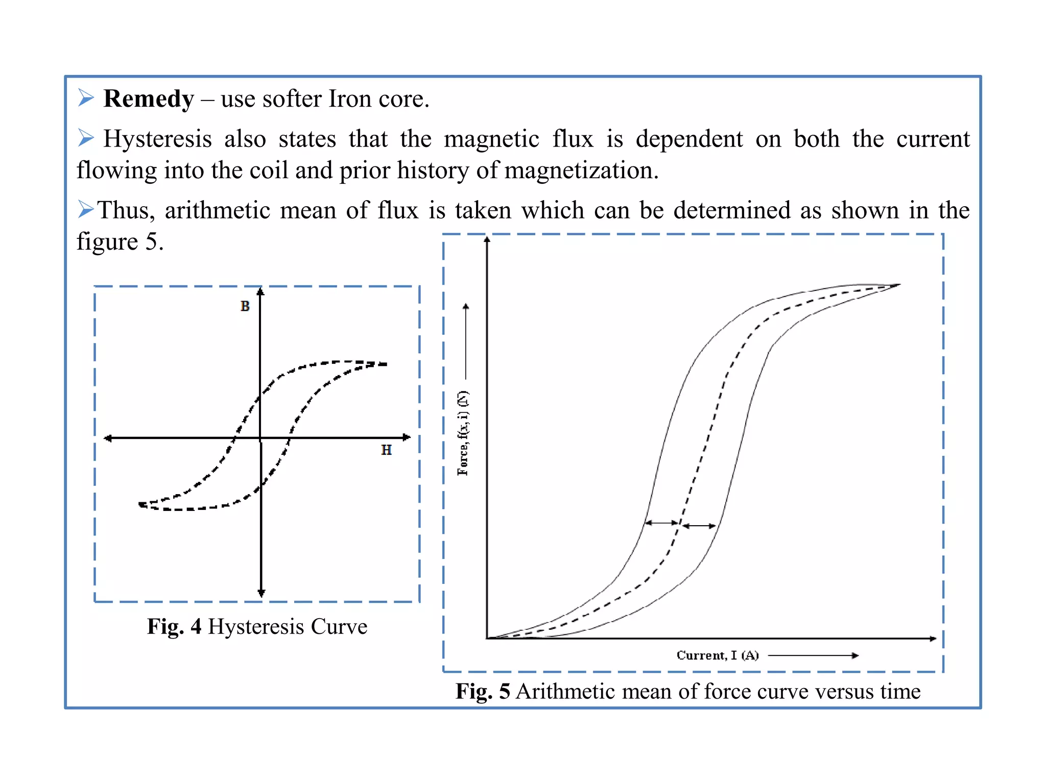
![4.1. General State-Space Transformation
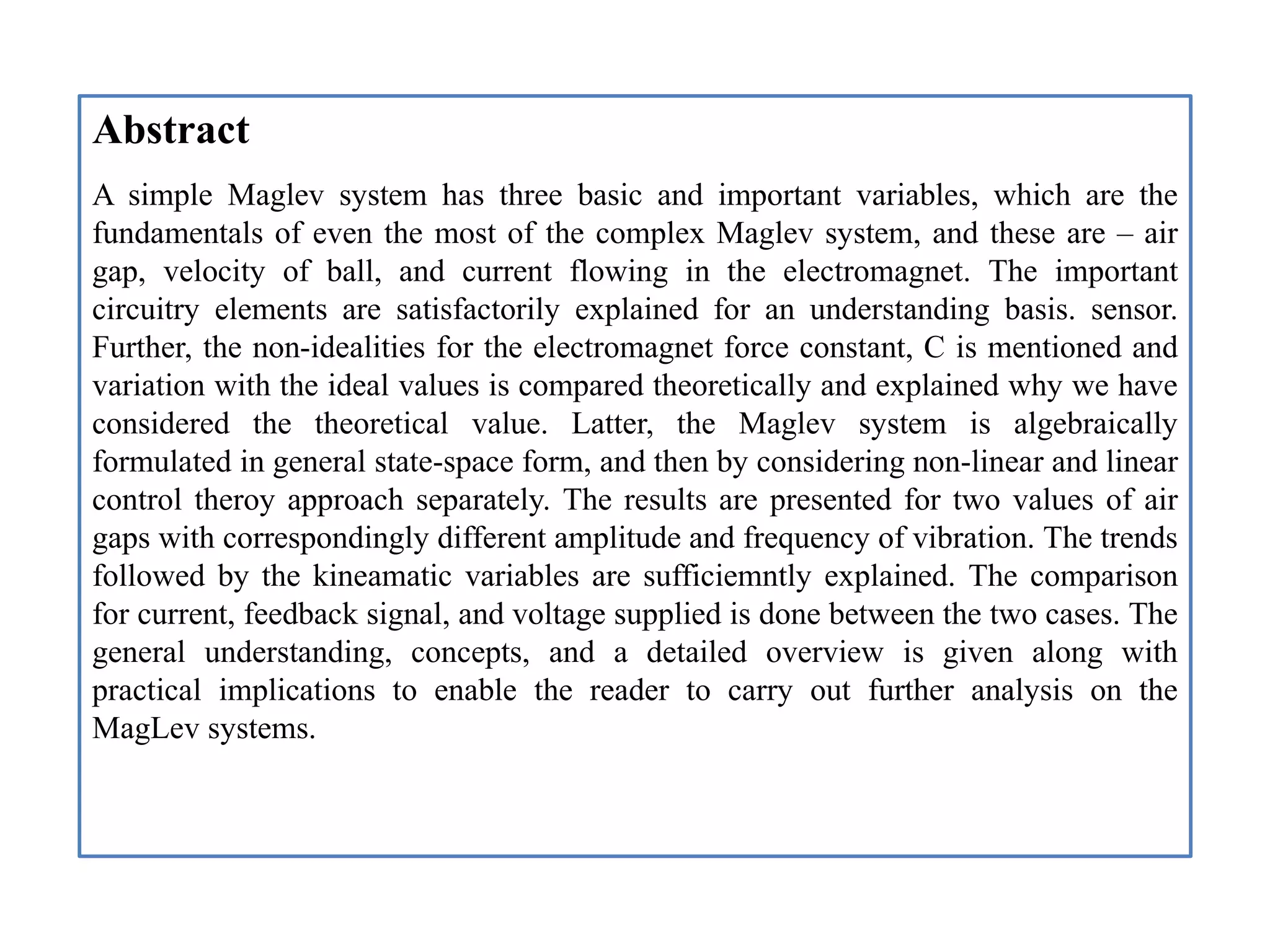
Using the fundamental principle of dynamics,
We know from the law of mutual inductance that
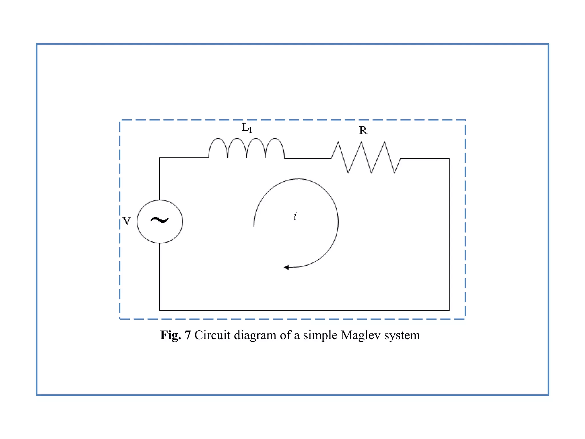
A simple circuit diagram of the maglev system is shown in Figure 7. Applying
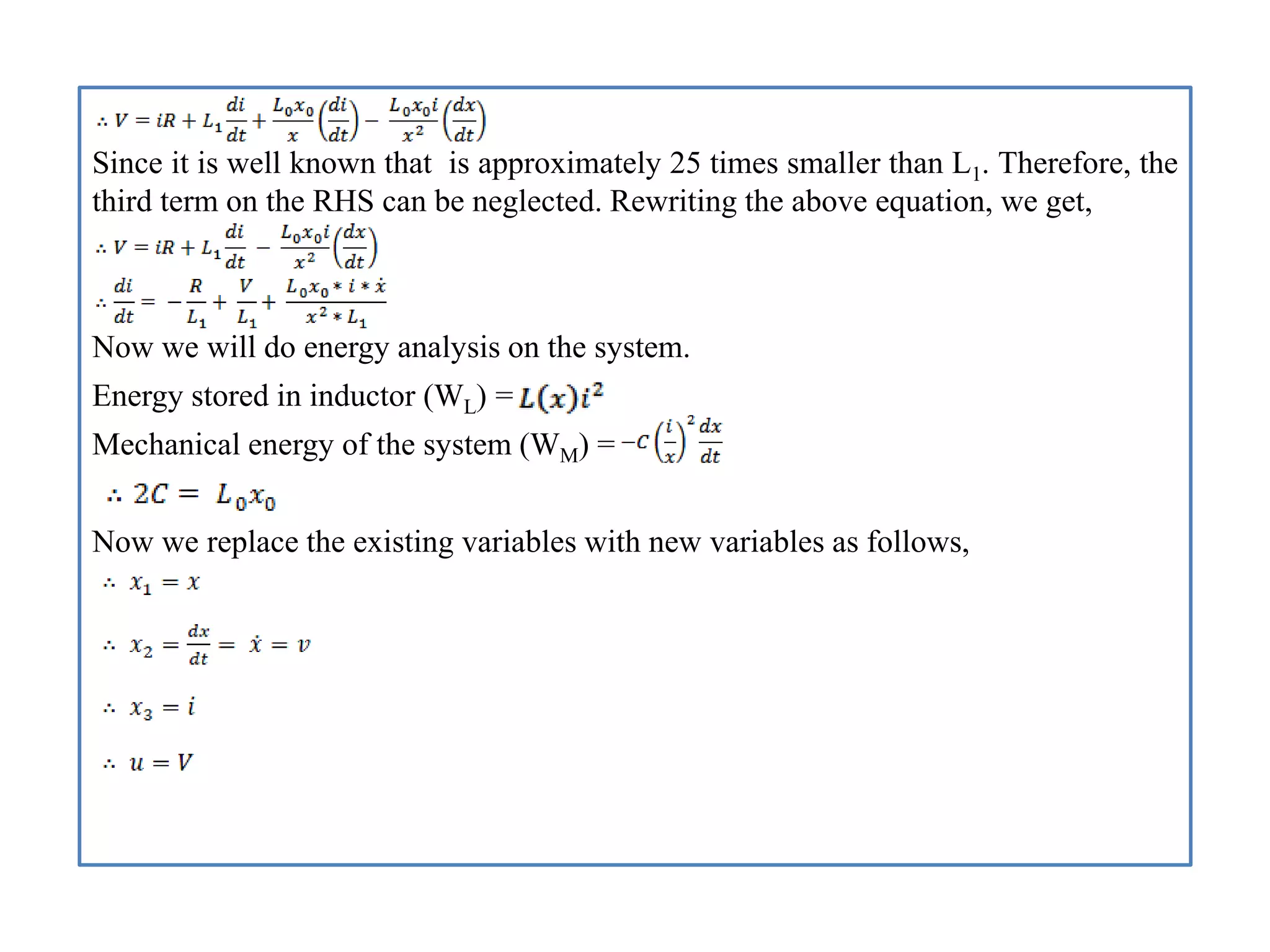
Kirchhoff's voltage law, we get,
As per Wong [2] the inductance is assumed to vary inversely with respect to ball's
position x.
Where x0 is the correction constant to incorporate the non-idealities in permeability.](https://image.slidesharecdn.com/presentationppt-180823175017/75/Analysis-of-Simple-Maglev-System-using-Simulink-15-2048.jpg)
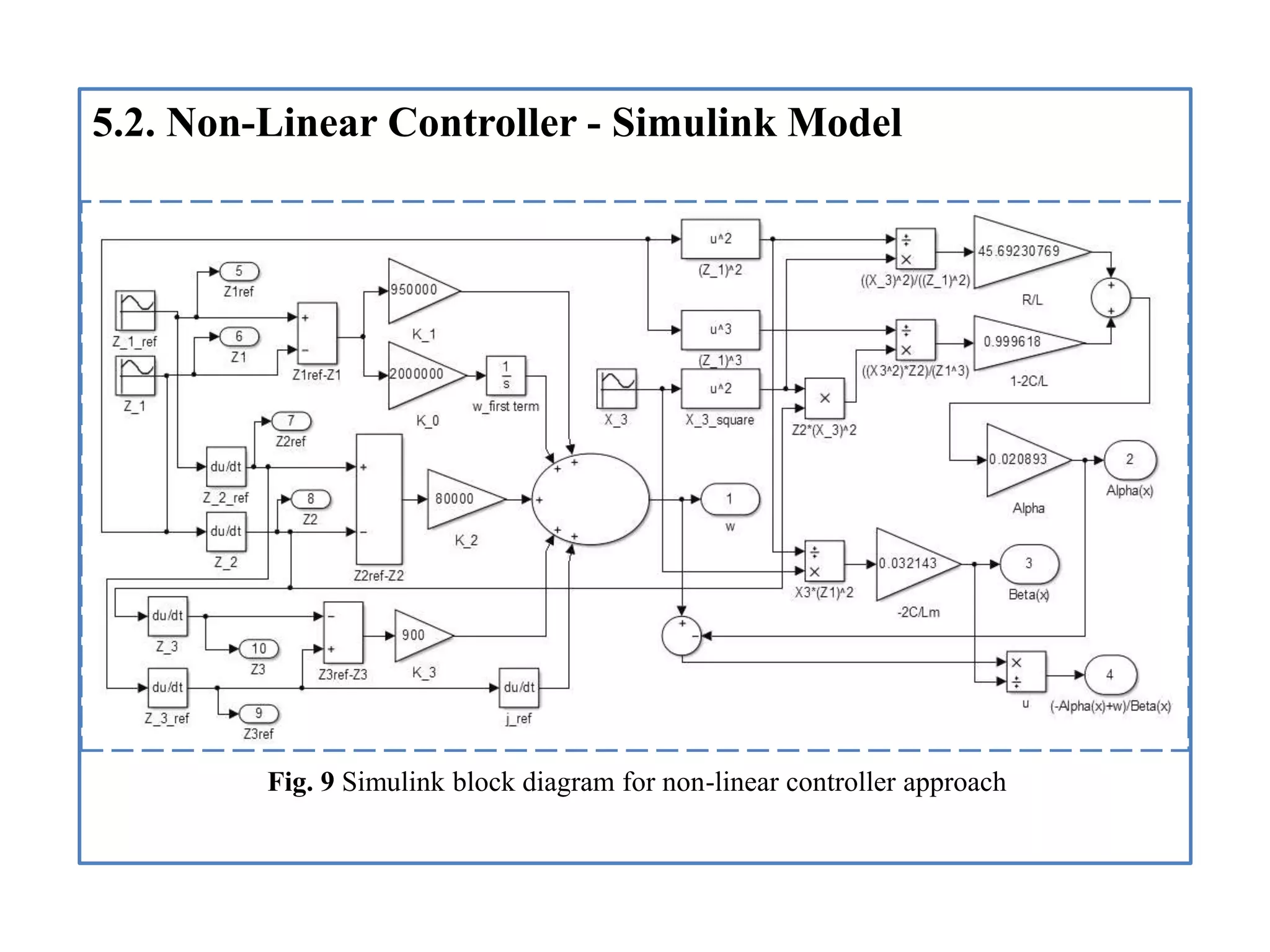
![4.2. Non-Linear Controller Approach
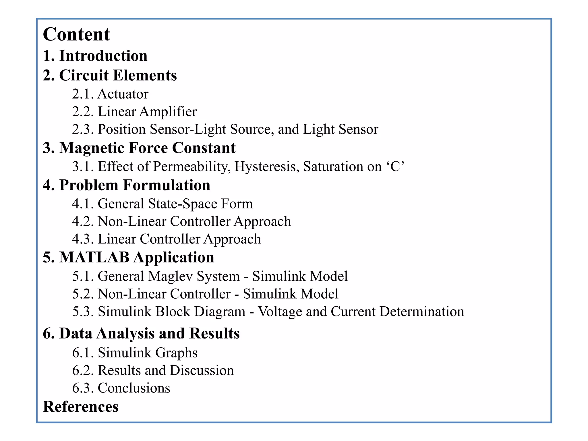
The assumption made in this approach constraints current and position are to always
have positive values which confirms that our transformation will be invertible [3].
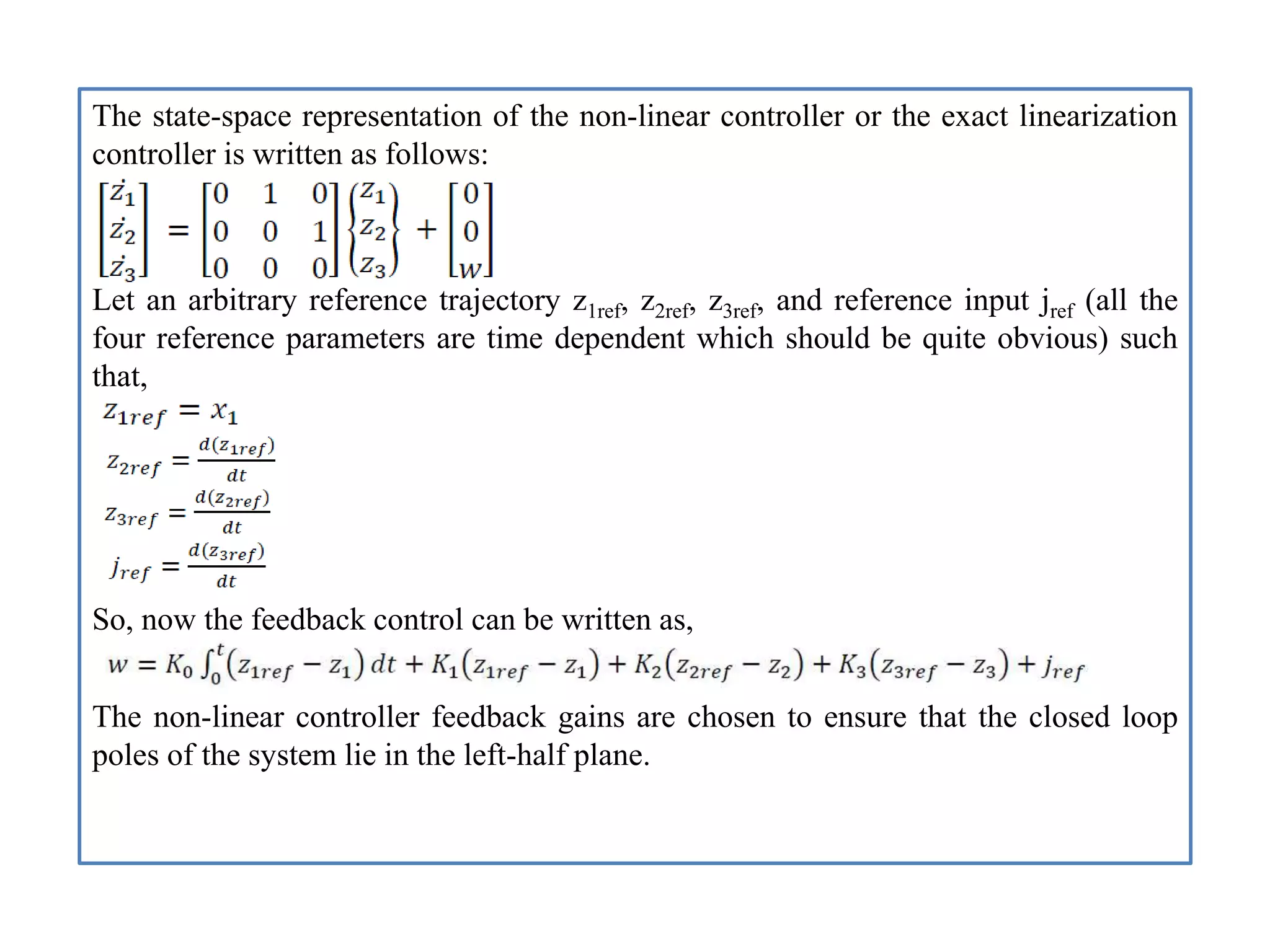
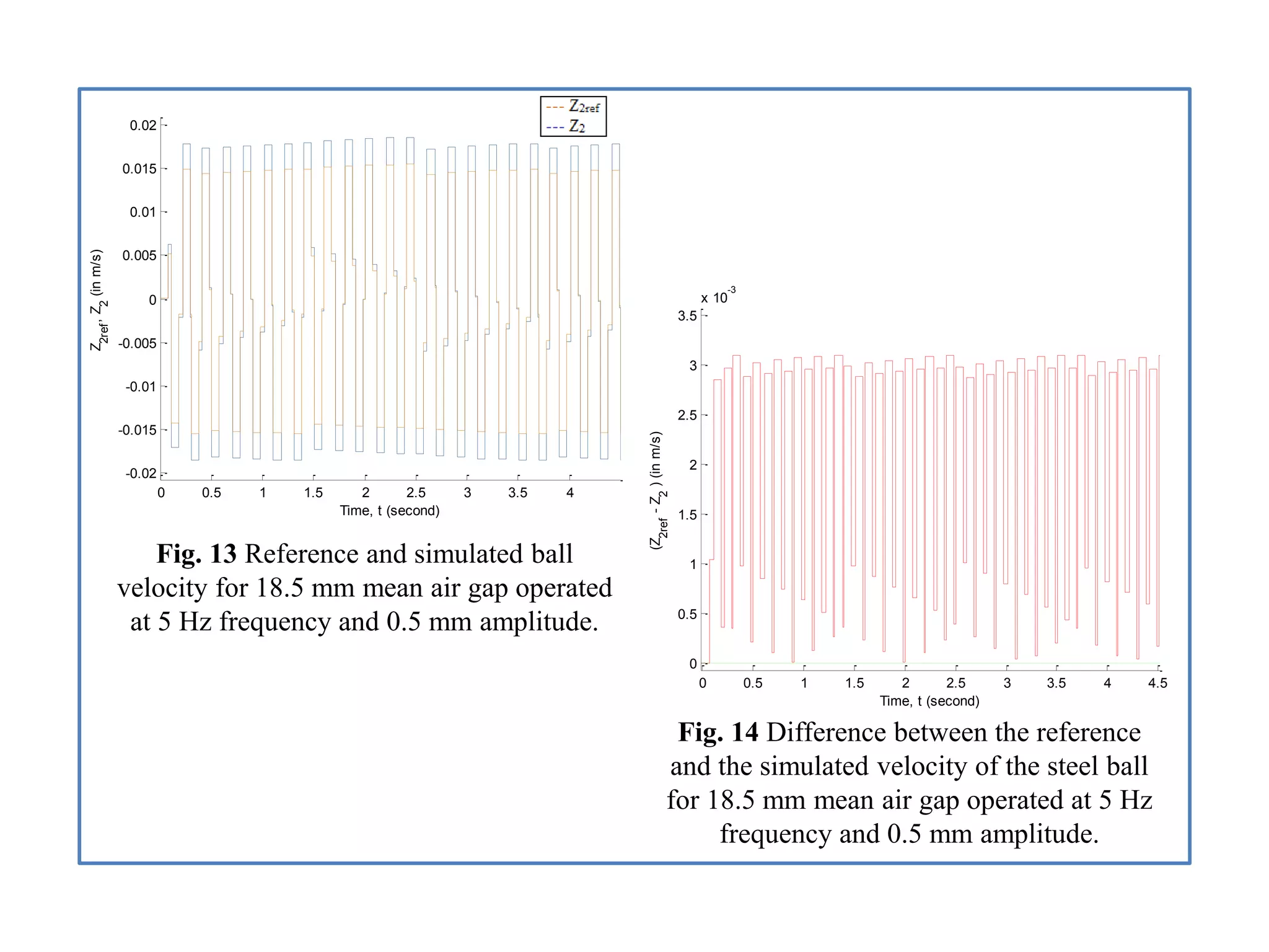
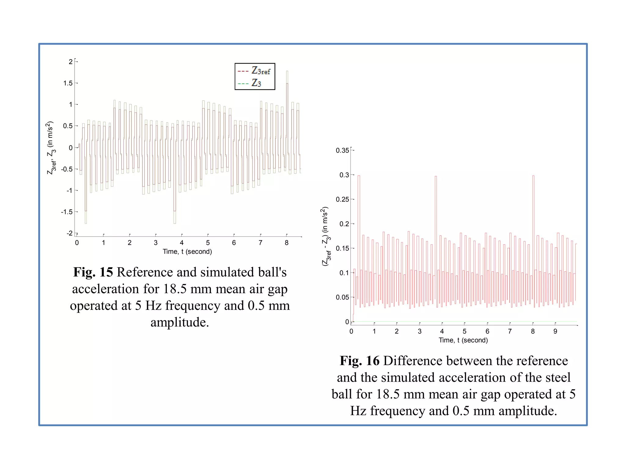
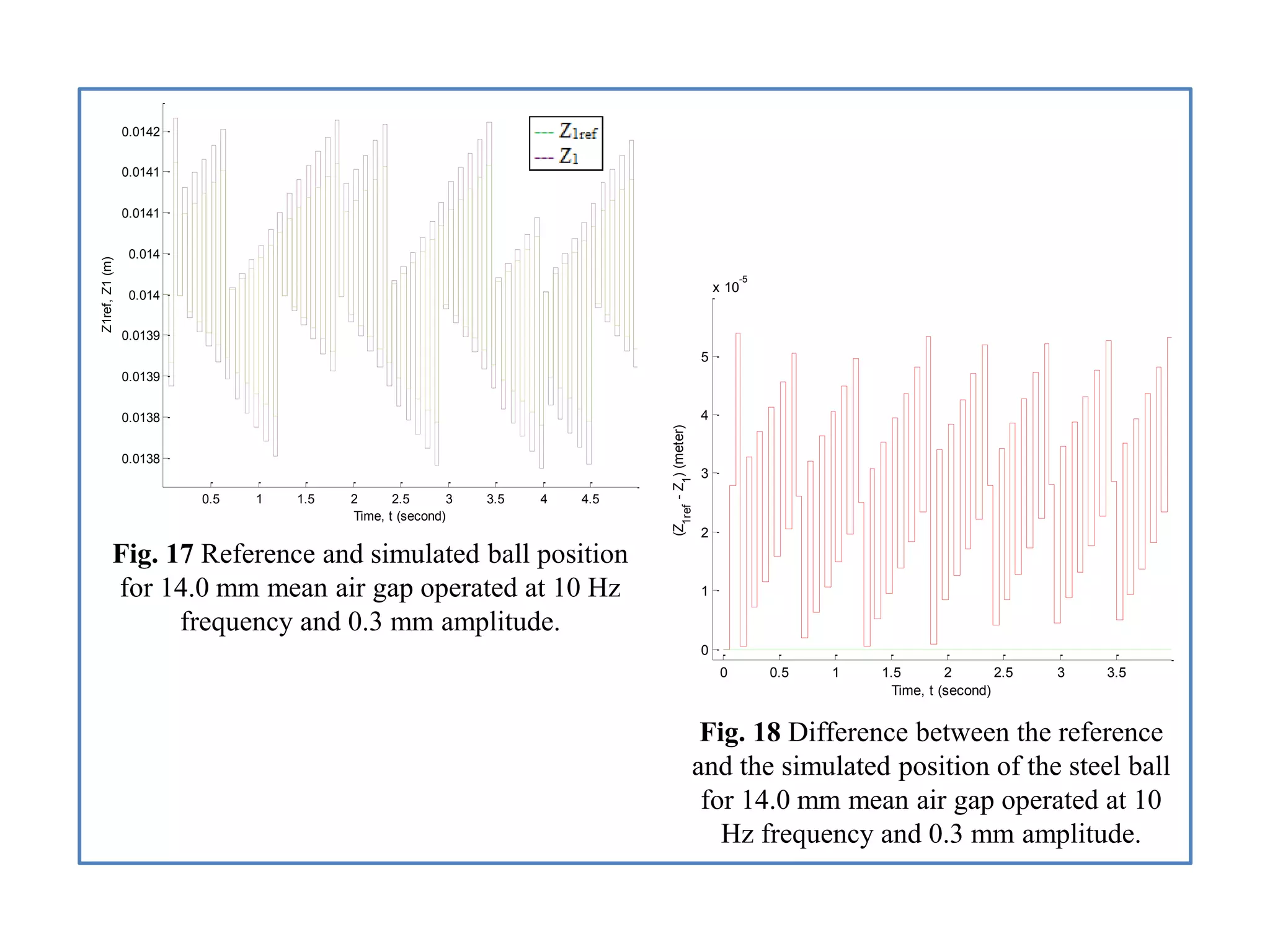
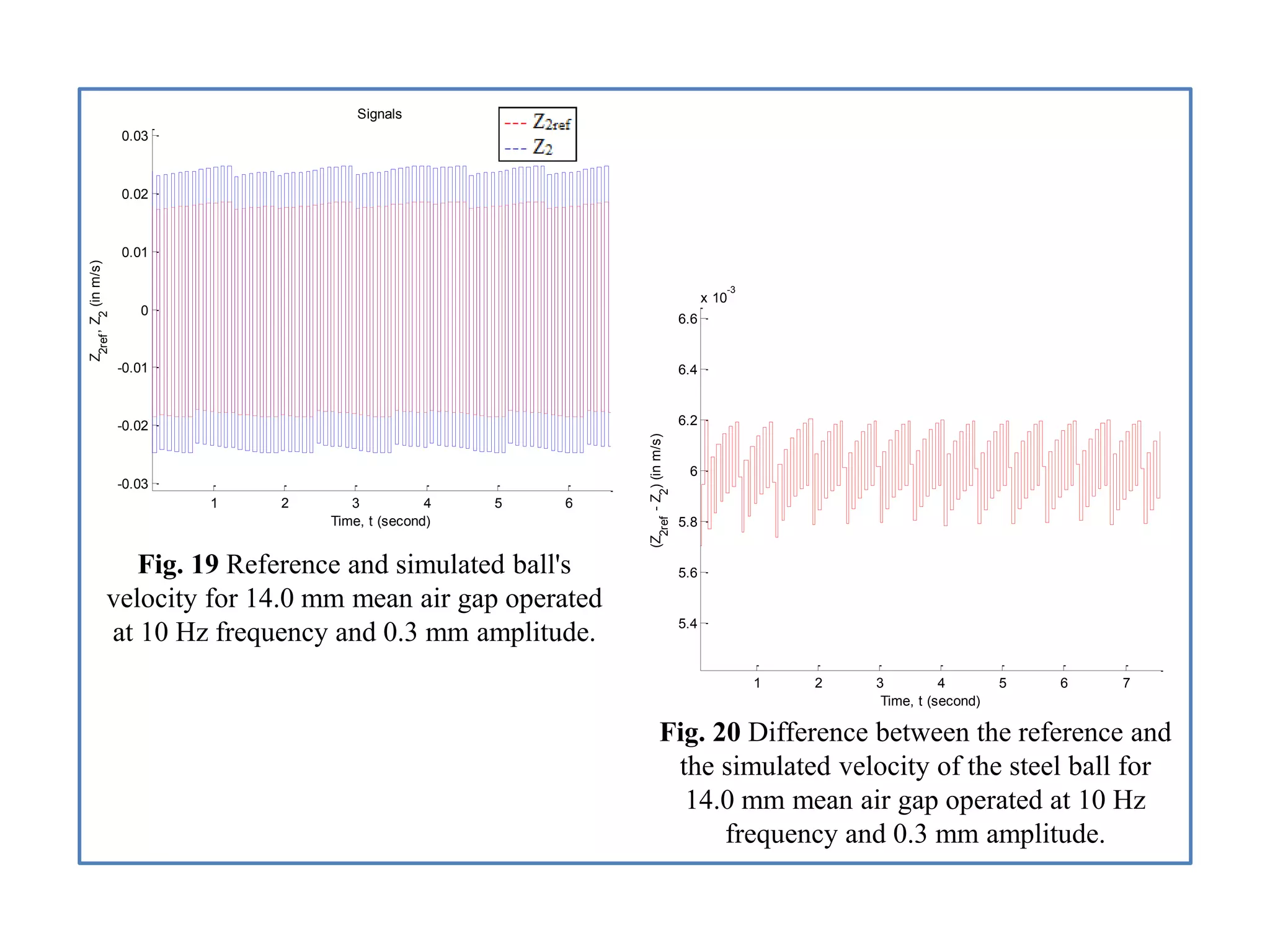
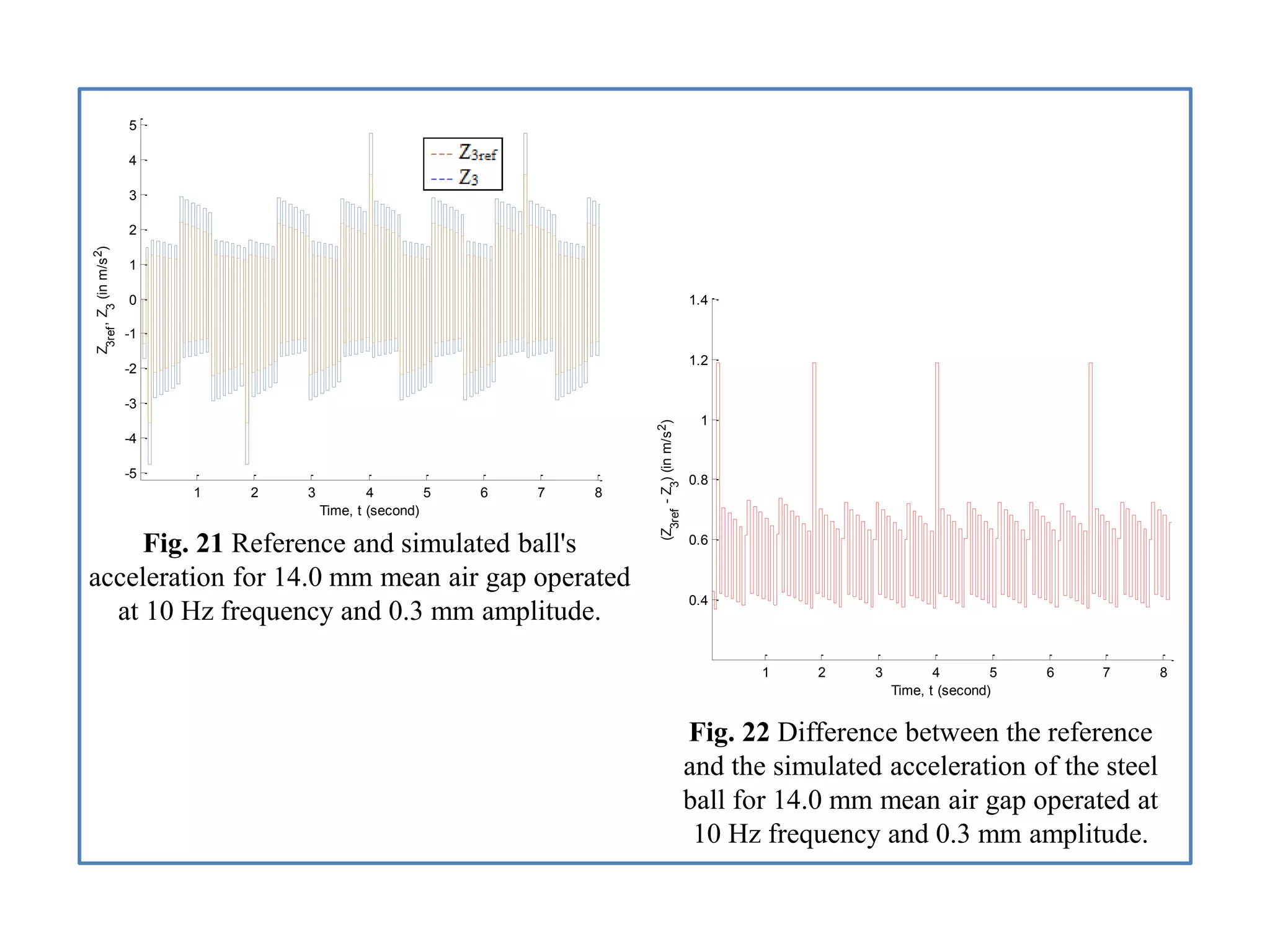
Let new state variables be Z1, Z2, and Z3 denoting the the levitated ball's position,
velocity and acceleration respectively. Thus now, we can write the transformation as,
According to the state feedback control,
, and
Where,
[4]
[4]](https://image.slidesharecdn.com/presentationppt-180823175017/75/Analysis-of-Simple-Maglev-System-using-Simulink-18-2048.jpg)
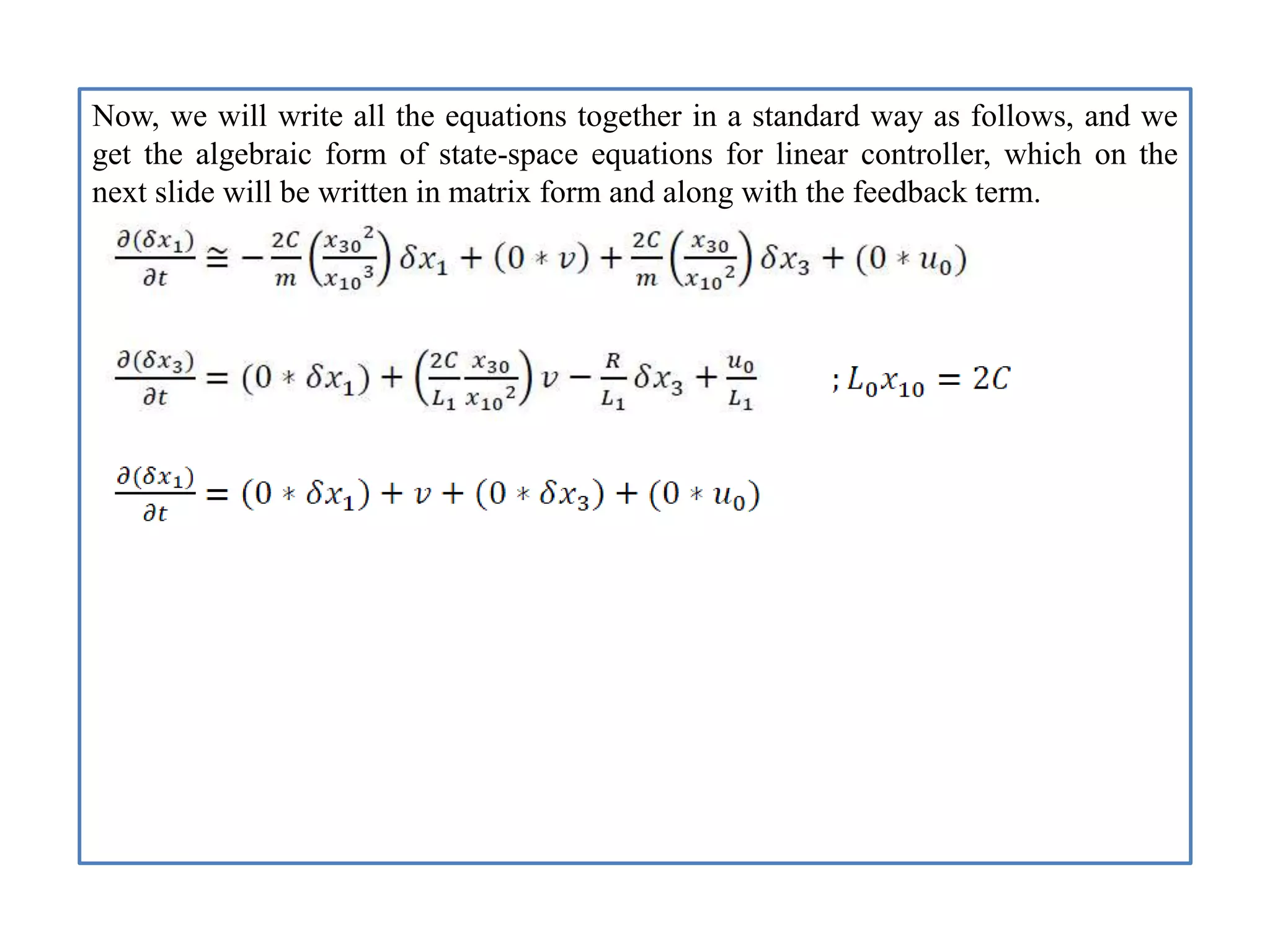
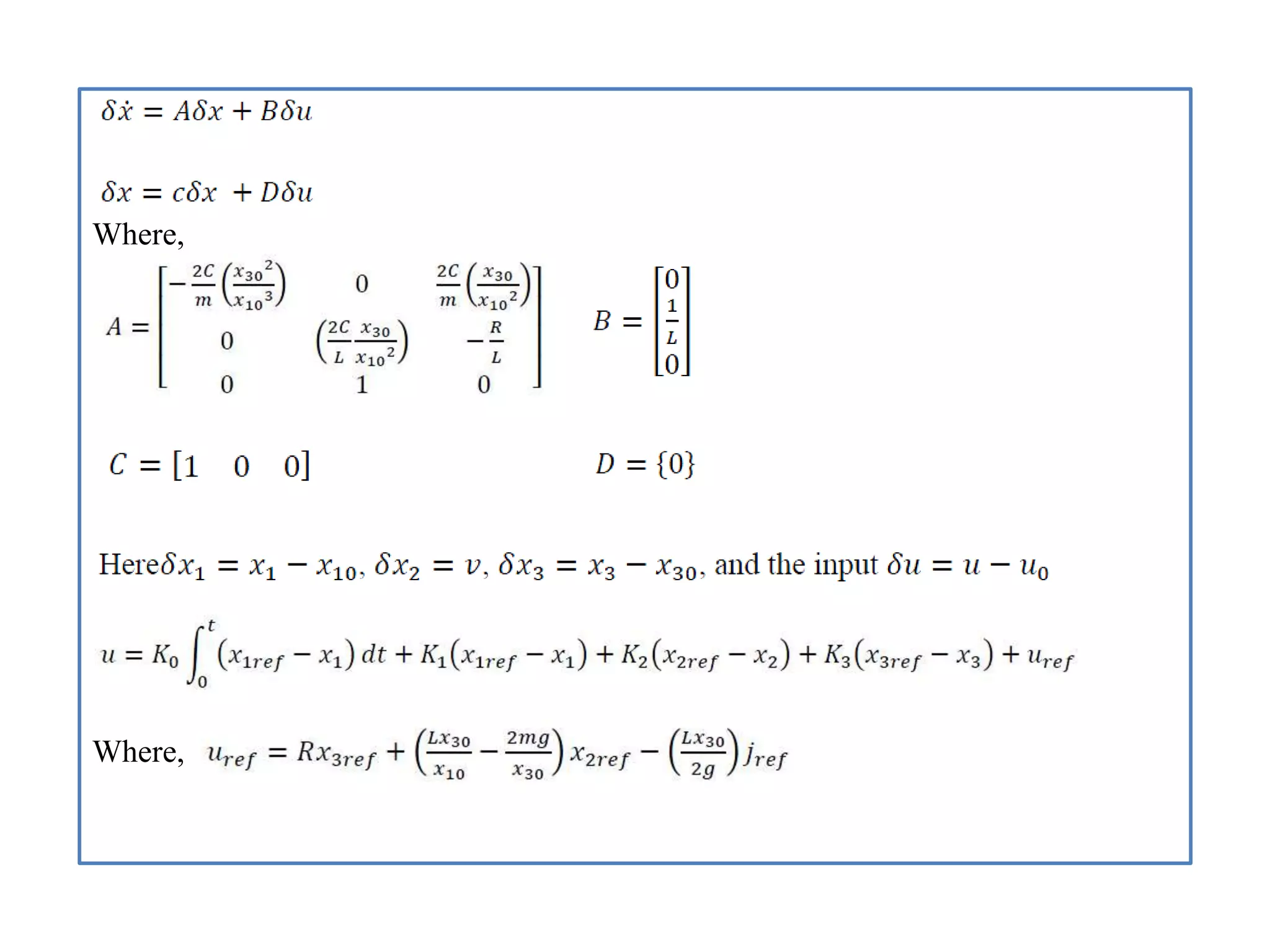
![4.3. Linear Controller Approach
Cho et al. [4] did a comparison of sliding mode controller versus a linear controller.
They proved a better response from a sliding mode controller than the linear
controller. The MagLev system can be linearized by using the following
procedure[6]. Consider a nominal input voltage u0 producing nominal current x30=i0,
which levitates the ball to the equilibrium position x10=x0 and x20=v=0.
Using the Taylor's series expansion , we get,
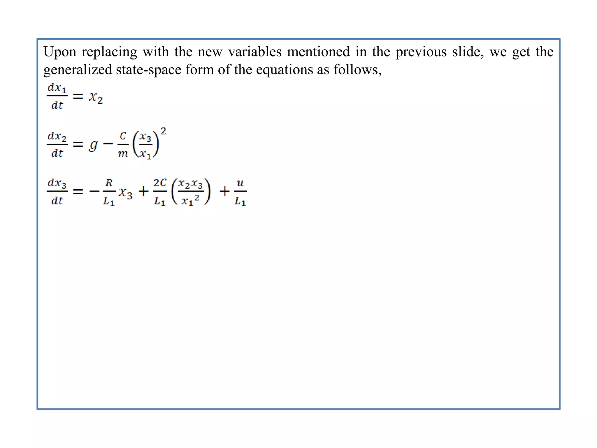
Using above equations in the generalized state-space equation, we get,
At nominal operating point,
, and
Therefore,](https://image.slidesharecdn.com/presentationppt-180823175017/75/Analysis-of-Simple-Maglev-System-using-Simulink-20-2048.jpg)
![References
[1] Siscoe, G. L. (1986). "An historical footnote on the origin of 'aurora
borealis'", History of Geophysics: Vol. 2,. p. 11. ISBN 0-87590-276-6.
[2] Wong,T., 1986, Design of a magnetic levitation system-an undergraduate
project, IEEE Transactions on Education, 29,196-200.
[3] Isidori, A., 1989, Nonlinear Control Systems, New York: Springer-Verlag.
[4] Krener, A., and Respondek, W., 1985, Nonlinear observers with
linearizable error dynamics, SIAM Journal on Control and Optimization.
[5] Cho, D., Kato, Y., Spilman, D., 1993, Experimental comparison of sliding
mode and classical controllers in magnetic levitation systems, IEEE
Control Systems.
[6] Krener, A., and Isidori, A., 1983, Linearization by output injection and
nonlinear observers, System and Control Letters, 3, 52-57.](https://image.slidesharecdn.com/presentationppt-180823175017/75/Analysis-of-Simple-Maglev-System-using-Simulink-41-2048.jpg)

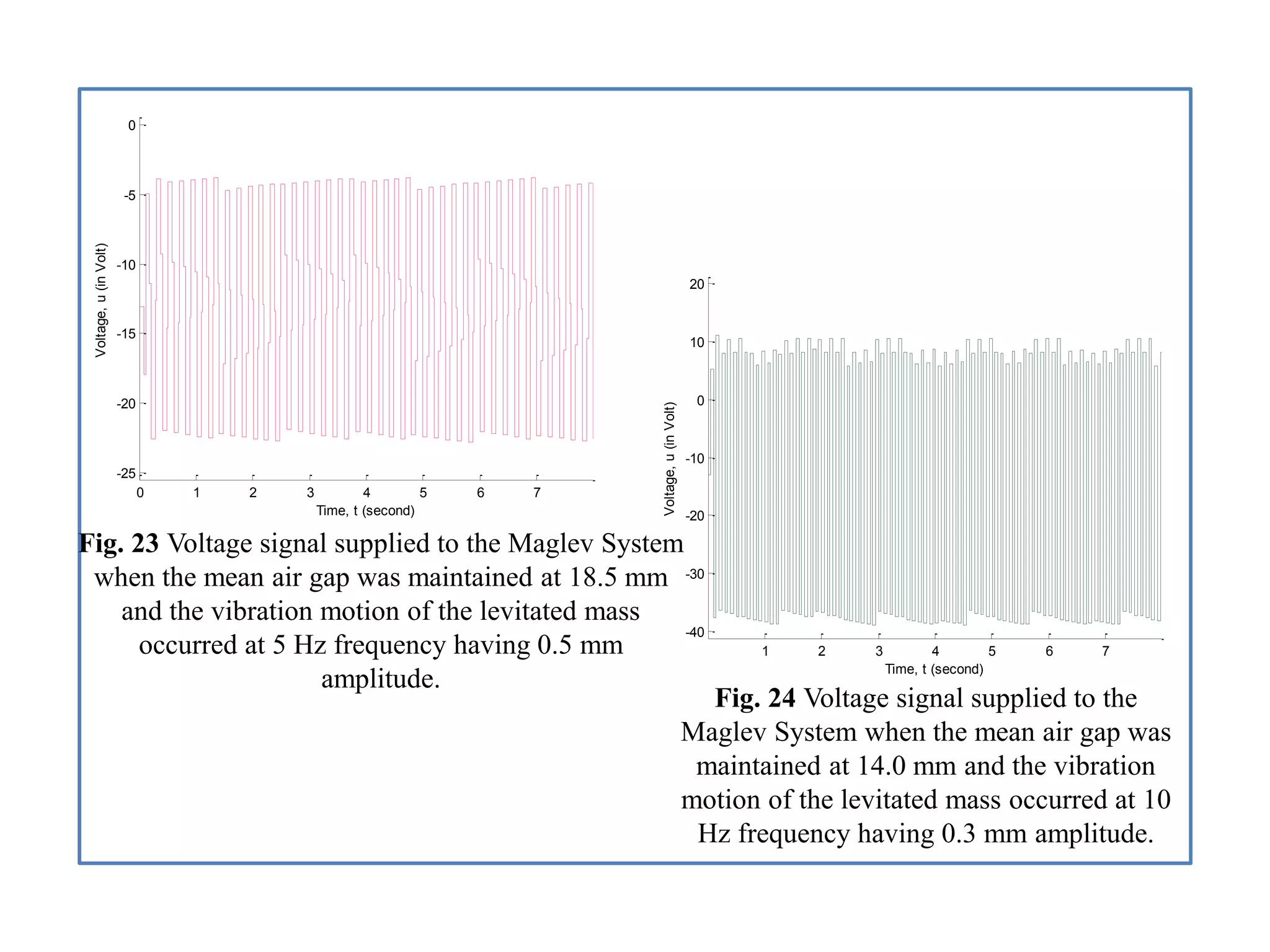
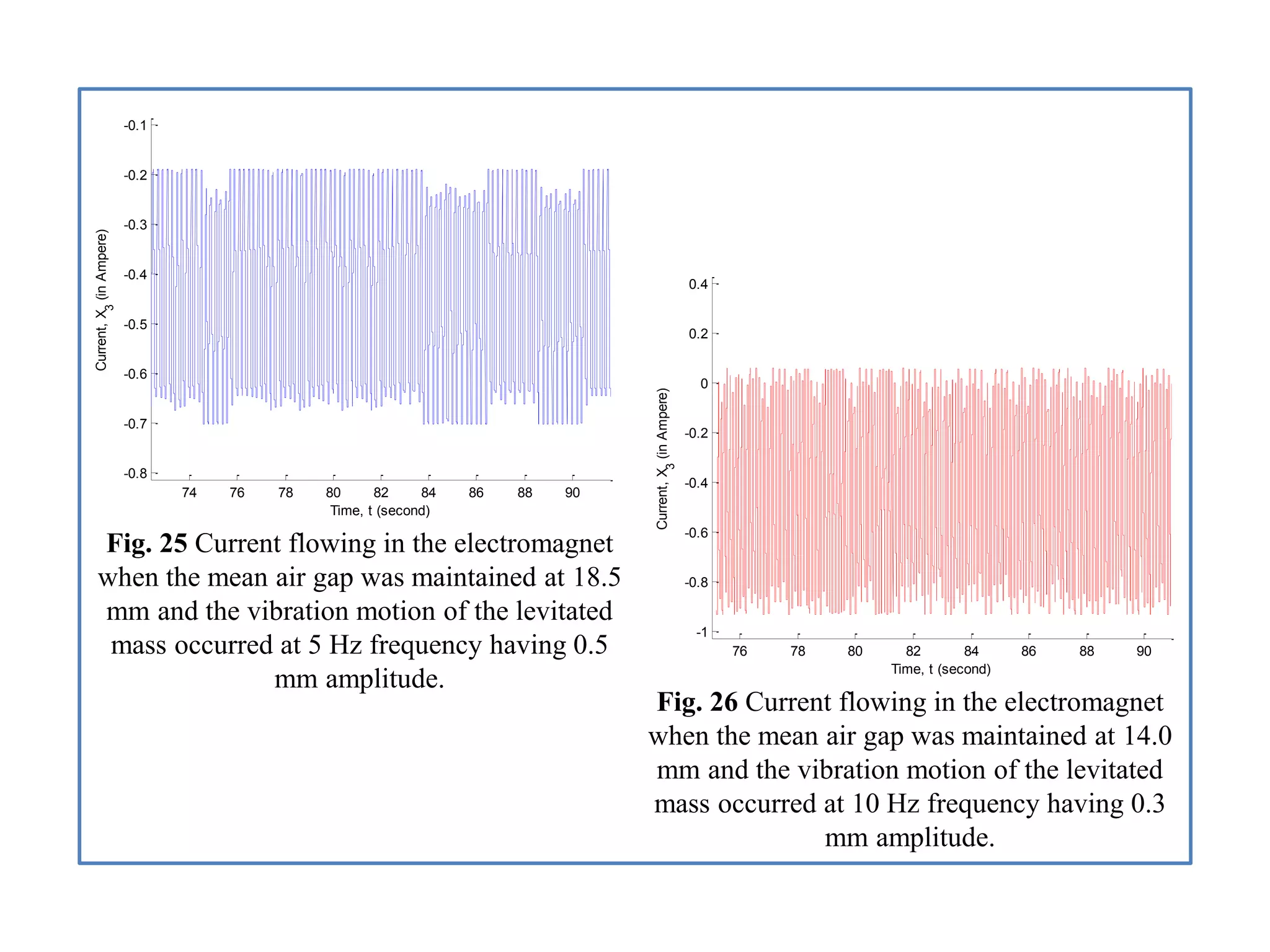
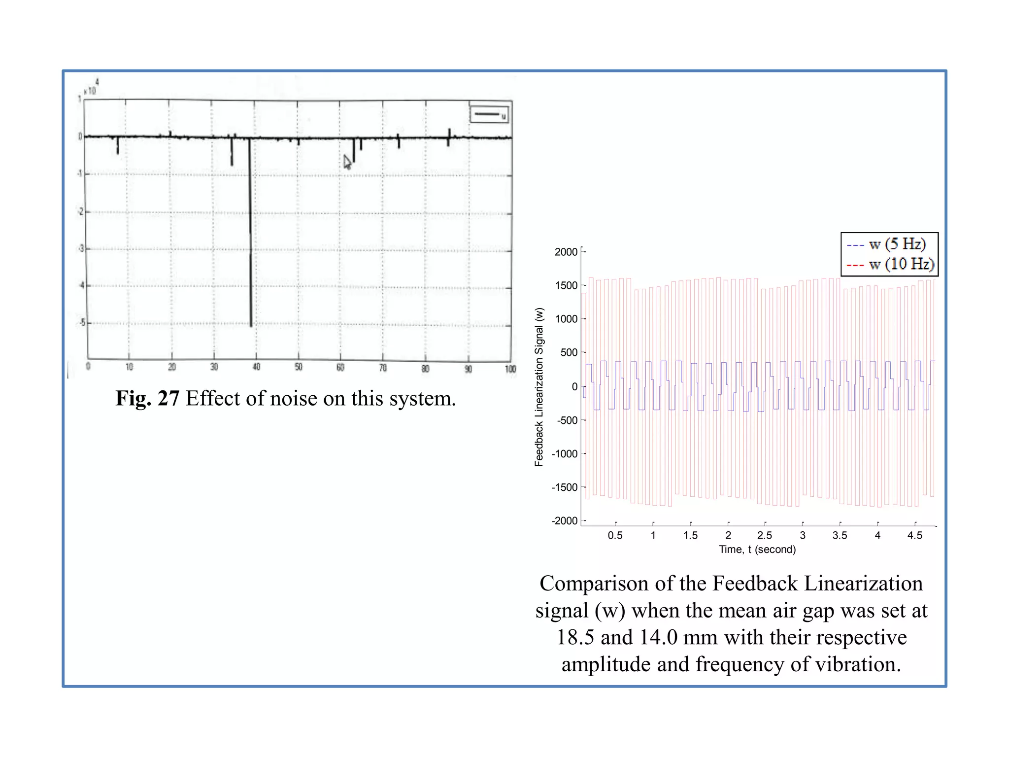
The document is a PowerPoint presentation analyzing a simple maglev system using Simulink. It includes: - An introduction to maglev systems and their applications. - Circuit diagrams and explanations of the position sensor, electromagnet actuator, and other system components. - Derivations of the system's mathematical model and equations in state space form for both nonlinear and linear controller approaches. - Descriptions of the Simulink models created to simulate the system, including blocks for the generalized system, nonlinear controller, and determining voltage and current. - Analysis of simulation results for two air gap scenarios, comparing graphs of position, velocity, acceleration, and other signals between the scenarios.


