The document presents a study investigating discrete quartic spline interpolation over non-uniform meshes. It begins with background on discrete splines and defines deficient splines. The paper then develops a new function for deficient quartic spline interpolation and obtains existence, uniqueness, and convergence properties of the deficient discrete quartic spline interpolation matching given function values at two interior points and first differences at midpoints, with boundary conditions on the function. It presents the analysis that leads to a system of equations and proves that for any mesh spacing h>0, there exists a unique deficient discrete quartic spline satisfying the given conditions.

1. Control Theory and Informatics www.iiste.org
ISSN 2224-5774 (Paper) ISSN 2225-0492 (Online)
Vol.4, No.6, 2014
1
The Discrete Quartic Spline Interpolation Over Non Uniform
Mesh
Y.P. Dubey K.K. Paroha
Department of Mathematics Gyan Ganga College of Technology
L.N.C.T. Jabalpur (M.P.)
Jabalpur(M.P.) India
India
E-mail: ypdubey2006@rediffmail.com E-mail parohakrishnakumar@rediffmail.com
ABSTRACT
The objective of the paper is to investigate precise error estimate concerning deficient
discrete quartic spline interpolation.
Mathematics subject classification code: 65D07
Key words: Deficient, Discrete, Quartic Spline, Interpolation, Error Bounds
1. ITNRODUCTION & PRILIMNARIES
Discrete Splines have been introduced by Mangasarian and Shumaker [5] in
connection with certain studied of minimization problems involving differences.
Deficient Spline are more useful then usual spline as they require less continuity
requirement at the mesh points. Malcolm [4] used discrete spline to compute non-
linear spline interactively. Discrete cubic splines which interpolate given functional
values at one intermediate point of a uniform mesh have been studied in [1]. These
results were generalized by Dikshit and Rana [2] for non-uniform meshes. Rana and
Dubey [8] have obtained local behavior of discrete cubic spline interpolation which is
some time used to smooth histogram. For some constructive aspect of discrete spline
reference may be made to Schumaker [3] and Jia [6].
We have develop a new function for deficient quartic spline interpolation .if we increase
the degree of polynomial with boundary condition, then we find that result is better
then by comparing with author [1, 2] for smoothness of the function.
In this paper, we have obtained existence, uniqueness and convergence properties of
deficient discrete quartic spline interpolation matching the given function at two

2. Control Theory and Informatics www.iiste.org
ISSN 2224-5774 (Paper) ISSN 2225-0492 (Online)
Vol.4, No.6, 2014
2
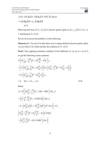
interior points of interval and first difference at mid points with boundary condition of
function.
Let us consider a mesh  on [0, 1] which is defined by
1......0: 10  nxxx
Such that iii Pxx  1 for i = 1, 2,...., n. Throughout h, will be represent a given
positive real number, consider a real continuous function ),( hxs defined over [0,1]
which is such that its restriction is on  ii xx ,1 is a polynomial of degree 4 or less for i
= 1,2,.....n then  hxs , defines a discrete deficient quartic spline if
    1,0,,_, 1
)()(
  jhxsDhxsD i
j
nii
j
n
(1.1)
Where the difference operator nD are defined as
       
h
hxfhxf
xfDxfxfD nn
2
)(, )1()0( 

The class of all discrete deficient quartic splines is denoted by  hS ,1,,4 
2. EXISTENCE AND UNIQUENESS
Consider the following conditions -
   ii fs   (2.1)
   ii fs   (2.2)
   i
j
hin sDsD  }{}1{
 (2.3)
for i = 1,2,.....n
Where iii Px
3
1
1  
iiii Px   
2
1
1
and boundary conditions
)()( 00 xfxs  (2.4)
   nn xfxs  (2.5)

3. Control Theory and Informatics www.iiste.org
ISSN 2224-5774 (Paper) ISSN 2225-0492 (Online)
Vol.4, No.6, 2014
3
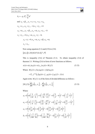
We shall prove the following.
Problem A : Given 0h for what restriction on iP does there exist a unique
   hPShxs ,,1,4,  which satisfy the condition (2.1) - (2.3) and boundary condition
(2.4)-(2.5).
Proof : Denoting
i
i
P
xx 
by t, 10 t . Let P(t) be a discrete quartic Polynomial on
[0,1], then we can show that
    


















2
1
2
1
3
1
)( }1{
21 PDtqPtqPtP h          tqPtqOPtq 543 1 (2.6)
Where
 
 





 

















 





 

9
1
,
36
1
18,
2
9
36,9
2
45
,
8
45
2
9
,
8
9 32
1
G
tGtGtGG
ttq
 
   





 











 








9
1
,
36
1
16,432,8
9
176
,
9
44
9
32
,
9
8 332
2
G
tGtGttGG
ttq
 





 

















 











 

9
1
,
36
1
0,
3
2
0,
9
11
0,
3
2
0,
9
1 32
3
G
tGtGtGG
ttq
 

















 








 











 





 


9
1
,
36
1
4,
3
1
8,
9
7
9
47
,
36
23
3
4
,
9
2
1 432
4
G
tGtGtGtG
tq
 





 























 







9
1
,
36
1
2,
6
1
4,
9
2
12
7
,
18
41
18
7
,
72
1 32
5
G
tGtGtGGt
tq
Where   babhabaG ,,, 2
 are real numbers? We can write (2.6) in the form of the
restriction  hxsi , of the deficient discrete quartic spline  hxs , on  1, ii xx as follows
:

4. Control Theory and Informatics www.iiste.org
ISSN 2224-5774 (Paper) ISSN 2225-0492 (Online)
Vol.4, No.6, 2014
4
            )(3
}1{
21 tqfDPtqftqfxs ihiiii  
       tqxstqxs ii 514 
(2.7)
Observing that from (2.7),  hxsi , is discrete quartic spline on  1, ii xx for i=1,2,...n-
1. Satisfying (2.1) - (2.5).
We are set to answer the problem A in the following:
Theorem 2.1 : For any h>0, then there exist a unique deficient discrete quartic spline
),,1,4(),( hPShxs  which satisfies the condition (2.1) - (2.5).
Proof : Now applying continuity condition of first difference of ),( hxs at ix in (2.7)
we get the following system equations.
1
22
1
3
8,
9
89
9
10
,
18
1
 
















 
iii shGPGP
iiiii sGPGPGPGP 






















 


















  8,
9
7
3
4
,
9
2
4,
9
4
6
1
,
24
1 23
1
2
1
3
1
23
1 4,
9
2
18
7
,
18
1



















 iii sGPGP
iF for i = 1,2,..... n-1 (2.8)
Where
   













 
  1
22
1
3
36,9
2
9
,
8
9
iiii fhGPGPF 
   1
22
1 32,8
9
32
,
9
8












 
 ii fGhPG 
  3
1
}1{22
11 0,
9
13
0,
9
2
 




















 iinii PfDhGPGP  ,
  ii fhGPG 22
32,
9
172
9
32
,
9
8














 
   














 ii fhGPG 22
36,9
2
9
,
2
9

5. Control Theory and Informatics www.iiste.org
ISSN 2224-5774 (Paper) ISSN 2225-0492 (Online)
Vol.4, No.6, 2014
5
 


















 
22}1{3
1 0,
9
11
0,
9
1
hGPGfDPP iihii 
Writing iii mhmhxs  )(),( (Say) for all i we can easily see that excess of the absolute
value of the coefficient of im dominants the sum of the absolute value of the
coefficient of 1im and 1im in (2.8) under the condition theorem 2.1 and is given by
    










 





 
 
222
1
6
1
,
18
31
24,10
18
23
,
12
7
iii PGhGPGhT
Therefore, the coefficient matrix of the system of equation (2.6) is diagonally
dominant and hence invertible. Thus the system of equation has unique solution. This
complete proof of theorem 2.1.
3. ERROR BOUNDS :
Now system of equation (2.6) may be written as
FhMhA )(),( (3.1)
Where A(h) is coefficient matrix and )()( hmhM i . However as already shown in the
proof of theorem 2.1 A(h) is invertible. Denoting the inverse of )(hA by )(1
hA
we
note that max norm )(1
hA
satisfies the following inequality.
)()(1
hJhA 
(3.2)
Where    1
1max)(

 hThJ , for convenience we assume in this section that 1 = Nh
where N is positive integer, it is also assume that the mesh points }{ ix are such that
 hix 1,0 , for i = 0,1,..., n
Where discrete interval [0,1]h is the set of points }.....,,0{ Nhh for a function f and two
disjoint points 1x and 2x in its domain the first divided difference is defined by
     
21
21
21,
xx
xfxf
xx f


 (3.3)
For convenience we write }1{
f for fDn
}1{
and ),( Pfw for modulus of continuity of f,
the discrete norm of the function f over the interval [0, 1] is defined by
)(max
]1,0[
xff
x
 (3.4)

6. Control Theory and Informatics www.iiste.org
ISSN 2224-5774 (Paper) ISSN 2225-0492 (Online)
Vol.4, No.6, 2014
6
We shall obtain the following the bound of error function )(),()( xfhxsxe  over the
discrete interval  h1,0 .
Theorem 3.1 : Suppose ),( hxs is the discrete quartic splines of theorem 2.1 then
 PfwhPKxe ,),()( }1{
 (3.5)
   PfwhPKhJxe i ,),(')( }1{
 (3.6)
   hfwhPKxe ,),("' }1{
 (3.7)
Where ),(),,( 1
hPKhPK and ),(" hPK are positive function of P and h.
Proof : Equation (3.1) may be written as
)()()()().( fLfhAhFxehA iiii  (Say)
When iii fhxsxe  ),()( (3.8)
We need following Lemma due to Lyche [9,10] to estimate inequality (3.3).
Lemma 3.1 : Let  m
iia 1
and  n
jjb 1
be given sequence of non-negative real numbers
such that   ji ba then for any real value function f defined on discrete interval
h]1,0[ , we have
     

m
x
h
j
fjjjjfiii kk
yyybxxxa
1 1
1 ,...,...., 1010
 
!
1}1{
K
a
Khfw i
(3.9)
Where  hji kK
yx 1,0,  , for relevant values of i , j and k. We can write the equation (2.8)
is of the form of error function as follows:
1
22
1
3
8,
9
89
9
10
,
18
1
 
















 
iii ehGPGP





















 

3
1
22
1
3
4,
9
4
8
1
,
24
1
iii PhGPGP
iiiiii FPhGPGPehGPG 






































 
 1
223
1
22
4,
9
2
18
7
,
18
1
8,
9
7
3
4
,
9
2
1
22
1
3
8,
9
89
9
10
,
8
1


















 
 iii fhGPGP

7. Control Theory and Informatics www.iiste.org
ISSN 2224-5774 (Paper) ISSN 2225-0492 (Online)
Vol.4, No.6, 2014
7





















 
22
1
3
4,
9
4
6
1
,
24
1
hGPP ii




















 
 
223
1 8,
9
7
3
4
,
9
2
hGPGP ii
1
22
1
3
1 4,
9
2
18
7
,
18
1



















 iii fhGPGPf  fLi (Say) (3.10)
First we write )( fLi is in the form of divided difference and using Lemma of Lyche
[9, 10] , we get
   

5
1
5
1
}1{
1,)(
i j
jii baPfwfL (3.11)
Where   














 

5
1
5
1
2
1
3
1
23
1
3
1 6,
2
3
36
13
,
432
1
i j
iiji hGPPhGPPba +








 

23
1
3
8
,
27
40
hGPP ii

















 
  2,
2
1
36
17
,
144
17 22
11
3
11 GhPGPPa ii

















 
 
22
11
3
12 8,
9
5
9
10
,
18
1
hGPGPPa ii











 





 
 
3
10
,
3
4
27
16
,
27
4 23
13 GPGPPa iii

















 
 
223
14
3
8
,
27
4
27
7
,
108
1
hGPGPPa iii


















 
22
11
3
5 0,
9
13
0,
9
2
hGPGPPa iii

















 
 
22
11
3
1 6,
2
3
4
3
,
16
3
hGPGPPb iii












 
9
1
,
36
133
12 GPPb ii






 
9
1
,
12
13
1
3
3 GPPb ii
3
1
3
4
9
1


 ii PPb

8. Control Theory and Informatics www.iiste.org
ISSN 2224-5774 (Paper) ISSN 2225-0492 (Online)
Vol.4, No.6, 2014
8
23
15
9
11
hPpb ii 
and 01110 42211 , yyxxxx iji  
hxhxxx iii   131312 100
,, 
hyyyy iiii   1321111 0010
,,, 
,,, 011 5413 hyyhx iii   
iiii xxxhy   0101 5445 ,,,
151  ixx
Now using equation (3.1) and (3.9) in (3.8)
 PfwhPKhJxe i ,'),()()( 
This is inequality (3.6) of Theorem (3.1). To obtain inequality (3.4) of
theorem 3.1. Writing (2.6) in form of error functions as follows.
)()()()()()( 514 fMtaxetaxexe iii   (3.12)
Where )()()()()( 211 tqftqffM ii  
  )()()()( 5413
}1{
1 xffqftqftqfP iiii   
Again write )( fMi is of the form of divided difference as follows :
     

3
1
2
1
1010
,,)(
i j
fjjjfiiii yybxxafM (3.13)
Where








 





 
 2
1
4
15
,
16
15
4
3
,
16
3
tGtGPa i 







 






 43
3,
4
3
6,
3
2
tGtG








 





 
 2
2
18
47
,
12
23
3
2
,
9
1
tGtGPa i 













 
 43
2,
3
4
4,
18
7
tGtG






























 432
3 0,
3
2
0,
9
11
0,
3
2
0,
9
1
tGtGtGtGPa i





























 
 432
1 1,
12
1
2,
9
1
36
79
,
144
7
36
17
,
144
7
tGtGtGtGPb i

9. Control Theory and Informatics www.iiste.org
ISSN 2224-5774 (Paper) ISSN 2225-0492 (Online)
Vol.4, No.6, 2014
9







9
1
,
9
5
2 GtPb i
By using Lemma 3.1 of Lyche [9.10]
  














 

3
1
2
1
2
36
41
,
144
7
12
1
,
144
5
i j
ji GttGba 














 43
1,
4
1
2,
9
2
tGtG
and
110 211 , xxx ii  
hxhxxx iii    100 3312 ,,
xyxyxyy iii   1010 21211 ,,,
From equation (3.6), (3.12) and (3.13) gives inequality (3.5) of Theorem 3.1.
We now proceed to obtain an upper bound of }1{
ie for we use first difference
operator in (2.6) equation we get
       fUtqetqexeAP iiiii  
}1{
5
}1{
41
}1{
(3.14)
Where          iiiii fPtqftqffU  }1{}1{
2
}1{
1)( 
       xfPtqftqftq iii
}1{}1{
5
}1{
41
}1{
3   A and 




 

9
1
,
36
1
GA
Now writing  fUi is of the form of divided difference. We get
       

3
1
2
1
1 1010
,,
i j
fjjjfiii yybxxafU
Where
 







 





 
 22
1 3
9
47
,
36
23
2
3
2
,
9
1
httGGPa i
  













 
2,
6
1
44,
6
59 22
GhttG
 







 






 22
2 3
18
59
,
72
7
2
36
7
,
144
1
htGtGPa i
 















 22
1,
12
1
42,
9
1
httGG

10. Control Theory and Informatics www.iiste.org
ISSN 2224-5774 (Paper) ISSN 2225-0492 (Online)
Vol.4, No.6, 2014
10
   





 2222
3
3
8
3
9
11
3
11
9
1
htthttPa i
 







 





 





 
 22
1 36,
2
3
2
15
,
8
15
2
4
3
,
16
3
htGtGPb i
  ,43,
4
3 22









 httG





 

9
1
,
36
1
2 GPb i
and hxyyy ii  010 211 ,, 
hxxxxhxy iii   0101 3112 ,,,
hxxxx iii    110 3122 ,,
Now, using Lemma 3.1 of Lyche [9,10] we get
   PfwbafU
i j
ji 







   
1,}1{
3
1
2
1
1 (3.15)
Where
  








 





 

3
1
2
1
1
2
15
,
8
15
2
36
31
,
8
105
i k
ij GGPba  22
3 ht 
  













 
3,
4
3
46,
2
3 22
GhttG
Now using equation (3.6), (3.14) and (3.15) we get inequality (3.7) of theorem
3.1. This complete proof of theorem 3.1.
Future scope: we have find out existence and uniqueness, error and convergence of
deficient discrete spline interpolation in interval [0, 1] by this spline method. The
deficient discrete quartic spline will match the function at two interior points and first
difference at middle point of the function with boundary condition.

11. Control Theory and Informatics www.iiste.org
ISSN 2224-5774 (Paper) ISSN 2225-0492 (Online)
Vol.4, No.6, 2014
11
REFERENCES
1. H.P. Dikshit and P. Powar. Discrete cubic spline interpolation. Numer. Math 40,
(1982), 71-79.
2. H.P. Dixit and S.S. Rana. Discrete cubic spline interpolation over a non-uniform
mesh, Rocky Mountain Jour. of Maths. 17, (1987), 709-718.
3. L.L. Schumaker. Construction aspects of discrete Polynomial Spline Function Approx.
Theory (G.G. Gorentz Ed.) Academic Press, New York (1973).
4. M.A. Malcololm, Non-Linear Function Report Stame, pp. 372-373 Stanford
University, 1973.
5. O.L. Mangasarian and L.L. Schumaker. Discrete Spline via Mathematical
Programming SIAM Jour. Control 9 (1971), 174-183.
6. Rong , Qing Jia , Total Positivity of the Discrete Spline Collocation matrix, J. approx.
theory, 39 (1983), 11-23.
7. S.S. Rana and Y.P. Dubey. Local behavior of the deficient discrete cubic spline
interpolation. J. Approx. Theory 86 (1996), 120-127.
8. S.S. Rana, Y.P. Dubey and R.K. Dubey. The deficient discrete quartic spline
interpolation, Jour. of Applied Math. and Bioinformatics, Vol. 4, No. 1 (2014), 21-32.
9. T. Lyche. Discrete Cubic Spline Interpolation, Report RRS University of Cyto 1975.
10. T. Lyche. Discrete Cubic Spline Interpolation, BIT, 16 (1976), 281-290.

12. The IISTE is a pioneer in the Open-Access hosting service and academic event
management. The aim of the firm is Accelerating Global Knowledge Sharing.
More information about the firm can be found on the homepage:
http://www.iiste.org
CALL FOR JOURNAL PAPERS
There are more than 30 peer-reviewed academic journals hosted under the hosting
platform.
Prospective authors of journals can find the submission instruction on the
following page: http://www.iiste.org/journals/ All the journals articles are available
online to the readers all over the world without financial, legal, or technical barriers
other than those inseparable from gaining access to the internet itself. Paper version
of the journals is also available upon request of readers and authors.
MORE RESOURCES
Book publication information: http://www.iiste.org/book/
IISTE Knowledge Sharing Partners
EBSCO, Index Copernicus, Ulrich's Periodicals Directory, JournalTOCS, PKP Open
Archives Harvester, Bielefeld Academic Search Engine, Elektronische
Zeitschriftenbibliothek EZB, Open J-Gate, OCLC WorldCat, Universe Digtial
Library , NewJour, Google Scholar

13. Business, Economics, Finance and Management Journals PAPER SUBMISSION EMAIL
European Journal of Business and Management EJBM@iiste.org
Research Journal of Finance and Accounting RJFA@iiste.org
Journal of Economics and Sustainable Development JESD@iiste.org
Information and Knowledge Management IKM@iiste.org
Journal of Developing Country Studies DCS@iiste.org
Industrial Engineering Letters IEL@iiste.org
Physical Sciences, Mathematics and Chemistry Journals PAPER SUBMISSION EMAIL
Journal of Natural Sciences Research JNSR@iiste.org
Journal of Chemistry and Materials Research CMR@iiste.org
Journal of Mathematical Theory and Modeling MTM@iiste.org
Advances in Physics Theories and Applications APTA@iiste.org
Chemical and Process Engineering Research CPER@iiste.org
Engineering, Technology and Systems Journals PAPER SUBMISSION EMAIL
Computer Engineering and Intelligent Systems CEIS@iiste.org
Innovative Systems Design and Engineering ISDE@iiste.org
Journal of Energy Technologies and Policy JETP@iiste.org
Information and Knowledge Management IKM@iiste.org
Journal of Control Theory and Informatics CTI@iiste.org
Journal of Information Engineering and Applications JIEA@iiste.org
Industrial Engineering Letters IEL@iiste.org
Journal of Network and Complex Systems NCS@iiste.org
Environment, Civil, Materials Sciences Journals PAPER SUBMISSION EMAIL
Journal of Environment and Earth Science JEES@iiste.org
Journal of Civil and Environmental Research CER@iiste.org
Journal of Natural Sciences Research JNSR@iiste.org
Life Science, Food and Medical Sciences PAPER SUBMISSION EMAIL
Advances in Life Science and Technology ALST@iiste.org
Journal of Natural Sciences Research JNSR@iiste.org
Journal of Biology, Agriculture and Healthcare JBAH@iiste.org
Journal of Food Science and Quality Management FSQM@iiste.org
Journal of Chemistry and Materials Research CMR@iiste.org
Education, and other Social Sciences PAPER SUBMISSION EMAIL
Journal of Education and Practice JEP@iiste.org
Journal of Law, Policy and Globalization JLPG@iiste.org
Journal of New Media and Mass Communication NMMC@iiste.org
Journal of Energy Technologies and Policy JETP@iiste.org
Historical Research Letter HRL@iiste.org
Public Policy and Administration Research PPAR@iiste.org
International Affairs and Global Strategy IAGS@iiste.org
Research on Humanities and Social Sciences RHSS@iiste.org
Journal of Developing Country Studies DCS@iiste.org
Journal of Arts and Design Studies ADS@iiste.org