![arXiv:math/0404188v6[math.NT]23Sep2007
THE PRIMES CONTAIN ARBITRARILY LONG ARITHMETIC
PROGRESSIONS
BEN GREEN AND TERENCE TAO
Abstract. We prove that there are arbitrarily long arithmetic progressions of primes.
There are three major ingredients. The first is Szemer´edi’s theorem, which asserts
that any subset of the integers of positive density contains progressions of arbitrary
length. The second, which is the main new ingredient of this paper, is a certain trans-
ference principle. This allows us to deduce from Szemer´edi’s theorem that any subset
of a sufficiently pseudorandom set (or measure) of positive relative density contains
progressions of arbitrary length. The third ingredient is a recent result of Goldston
and Yıldırım, which we reproduce here. Using this, one may place (a large fraction
of) the primes inside a pseudorandom set of “almost primes” (or more precisely, a
pseudorandom measure concentrated on almost primes) with positive relative density.
1. Introduction
It is a well-known conjecture that there are arbitrarily long arithmetic progressions
of prime numbers. The conjecture is best described as “classical”, or maybe even
“folklore”. In Dickson’s History it is stated that around 1770 Lagrange and Waring
investigated how large the common difference of an arithmetic progression of L primes
must be, and it is hard to imagine that they did not at least wonder whether their
results were sharp for all L.
It is not surprising that the conjecture should have been made, since a simple heuristic
based on the prime number theorem would suggest that there are ≫ N2
/ logk
N k-
tuples of primes p1, . . . , pk in arithmetic progression, each pi being at most N. Hardy and
Littlewood [24], in their famous paper of 1923, advanced a very general conjecture which,
as a special case, contains the hypothesis that the number of such k-term progressions
is asymptotically CkN2
/ logk
N for a certain explicit numerical factor Ck > 0 (we do
not come close to establishing this conjecture here, obtaining instead a lower bound
(γ(k) + o(1))N2
/ logk
N for some very small γ(k) > 0).
The first theoretical progress on these conjectures was made by van der Corput [42] (see
also [8]) who, in 1939, used Vinogradov’s method of prime number sums to establish the
case k = 3, that is to say that there are infinitely many triples of primes in arithmetic
progression. However, the question of longer arithmetic progressions seems to have
remained completely open (except for upper bounds), even for k = 4. On the other
hand, it has been known for some time that better results can be obtained if one
replaces the primes with a slightly larger set of almost primes. The most impressive
1991 Mathematics Subject Classification. 11N13, 11B25, 374A5.
While this work was carried out the first author was a PIMS postdoctoral fellow at the University of
British Columbia, Vancouver, Canada. The second author was a Clay Prize Fellow and was supported
by a grant from the Packard Foundation.
1](https://image.slidesharecdn.com/theprimescontainarbitrarilylongarithmeticprogressions-180218024935/85/Teorema-de-Green-Tao-1-320.jpg)
![2 BEN GREEN AND TERENCE TAO
such result is due to Heath-Brown [25]. He showed that there are infinitely many 4-term
progressions consisting of three primes and a number which is either prime or a product
of two primes. In a somewhat different direction, let us mention the beautiful results of
Balog [2, 3]. Among other things he shows that for any m there are m distinct primes
p1, . . . , pm such that all of the averages 1
2
(pi + pj) are prime.
The problem of finding long arithmetic progressions in the primes has also attracted the
interest of computational mathematicians. At the time of writing the longest known
arithmetic progression of primes is of length 23, and was found in 2004 by Markus Frind,
Paul Underwood, and Paul Jobling:
56211383760397 + 44546738095860k; k = 0, 1, . . ., 22.
An earlier arithmetic progression of primes of length 22 was found by Moran, Pritchard
and Thyssen [32]:
11410337850553 + 4609098694200k; k = 0, 1, . . ., 21.
Our main theorem resolves the above conjecture.
Theorem 1.1. The prime numbers contain infinitely many arithmetic progressions of
length k for all k.
In fact, we can say something a little stronger:
Theorem 1.2 (Szemer´edi’s theorem in the primes). Let A be any subset of the prime
numbers of positive relative upper density, thus lim supN→∞ π(N)−1
|A ∩ [1, N]| > 0,
where π(N) denotes the number of primes less than or equal to N. Then A contains
infinitely many arithmetic progressions of length k for all k.
If one replaces “primes” in the statement of Theorem 1.2 by the set of all positive integers
Z+
, then this is a famous theorem of Szemer´edi [38]. The special case k = 3 of Theorem
1.2 was recently established by the first author [21] using methods of Fourier analysis.
In contrast, our methods here have a more ergodic theory flavour and do not involve
much Fourier analysis (though the argument does rely on Szemer´edi’s theorem which
can be proven by either combinatorial, ergodic theory, or Fourier analysis arguments).
We also remark that if the primes were replaced by a random subset of the integers,
with density at least N−1/2+ε
on each interval [1, N], then the k = 3 case of the above
theorem was established in [30].
Acknowledgements The authors would like to thank Jean Bourgain, Enrico Bombieri,
Tim Gowers, Bryna Kra, Elon Lindenstrauss, Imre Ruzsa, Roman Sasyk, Peter Sarnak
and Kannan Soundararajan for helpful conversations. We are particularly indebted to
Andrew Granville for drawing our attention to the work of Goldston and Yıldırım, and to
Dan Goldston for making the preprint [17] available. We are also indebted to Yong-Gao
Chen and his students, Bryna Kra, Jamie Radcliffe, Lior Silberman and Mark Watkins
for corrections to earlier versions of the manuscript. We are particularly indebted to
the anonymous referees for a very thorough reading and many helpful corrections and
suggestions, which have been incorporated into this version of the paper. Portions of
this work were completed while the first author was visiting UCLA and Universit´e de
Montr´eal, and he would like to thank these institutions for their hospitality. He would
also like to thank Trinity College, Cambridge for support over several years.](https://image.slidesharecdn.com/theprimescontainarbitrarilylongarithmeticprogressions-180218024935/85/Teorema-de-Green-Tao-2-320.jpg)
![THE PRIMES CONTAIN ARBITRARILY LONG ARITHMETIC PROGRESSIONS 3
2. An outline of the proof
Let us start by stating Szemer´edi’s theorem properly. In the introduction we claimed
that it was a statement about sets of integers with positive upper density, but there are
other equivalent formulations. A “finitary” version of the theorem is as follows.
Proposition 2.1 (Szemer´edi’s theorem). [37, 38] Let N be a positive integer and let
ZN := Z/NZ.1
Let δ > 0 be a fixed positive real number, and let k 3 be an integer.
Then there is a minimal N0(δ, k) < ∞ with the following property. If N N0(δ, k) and
A ⊆ ZN is any set of cardinality at least δN, then A contains an arithmetic progression
of length k.
Finding the correct dependence of N0 on δ and k (particularly δ) is a famous open
problem. It was a great breakthrough when Gowers [18, 19] showed that
N0(δ, k) 22δ−ck
,
where ck is an explicit constant (Gowers obtains ck = 22k+9
). It is possible that a
new proof of Szemer´edi’s theorem could be found, with sufficiently good bounds that
Theorem 1.1 would follow immediately. To do this one would need something just a
little weaker than
N0(δ, k) 2ckδ−1
(2.1)
(there is a trick, namely passing to a subprogression of common difference 2 × 3 × 5 ×
· · · × w(N) for appropriate w(N), which allows one to consider the primes as a set of
density essentially log log N/ log N rather than 1/ log N; we will use a variant of this
“W-trick” later in this paper to eliminate local irregularities arising from small divisors).
In our proof of Theorem 1.2, we will need to use Szemer´edi’s theorem, but we will not
need any quantitative estimimates on N0(δ, k).
Let us state, for contrast, the best known lower bound which is due to Rankin [35] (see
also Lacey-Laba [31]):
N0(δ, k) exp(C(log 1/δ)1+⌊log2(k−1)⌋
).
At the moment it is clear that a substantial new idea would be required to obtain a result
of the strength (2.1). In fact, even for k = 3 the best bound is N0(δ, 3) 2Cδ−2 log(1/δ)
, a
result of Bourgain [6]. The hypothetical bound (2.1) is closely related to the following
very open conjecture of Erd˝os:
Conjecture 2.2 (Erd˝os conjecture on arithmetic progressions). Suppose that A = {a1 <
a2 < . . . } is an infinite sequence of integers such that 1/ai = ∞. Then A contains
arbitrarily long arithmetic progressions.
This would imply Theorem 1.1.
We do not make progress on any of these issues here. In one sentence, our argument can
be described instead as a transference principle which allows us to deduce Theorems
1We will retain this notation throughout the paper, thus ZN will never refer to the N-adics. We
always assume for convenience that N is prime. It is very convenient to work in ZN , rather than the
more traditional [−N, N], since we are free to divide by 2, 3, . . . , k and it is possible to make linear
changes of variables without worrying about the ranges of summation. There is a slight price to pay
for this, in that one must now address some “wraparound” issues when identifying ZN with a subset
of the integers, but these will be easily dealt with.](https://image.slidesharecdn.com/theprimescontainarbitrarilylongarithmeticprogressions-180218024935/85/Teorema-de-Green-Tao-3-320.jpg)
![4 BEN GREEN AND TERENCE TAO
1.1 and 1.2 from Szemer´edi’s theorem, regardless of what bound we know for N0(δ, k);
in fact we prove a more general statement in Theorem 3.5 below. Thus, in this paper,
we must assume Szemer´edi’s theorem. However with this one (rather large!) caveat2
our paper is self-contained.
Szemer´edi’s theorem can now be proved in several ways. The original proof of Szemer´edi
[37, 38] was combinatorial. In 1977, Furstenberg made a very important breakthrough
by providing an ergodic-theoretic proof [10]. Perhaps surprisingly for a result about
primes, our paper has at least as much in common with the ergodic-theoretic approach
as it does with the harmonic analysis approach of Gowers. We will use a language
which suggests this close connection, without actually relying explicitly on any ergodic-
theoretical concepts3
. In particular we shall always remain in the finitary setting of ZN ,
in contrast to the standard ergodic theory framework in which one takes weak limits
(invoking the axiom of choice) to pass to an infinite measure-preserving system. As will
become clear in our argument, in the finitary setting one can still access many tools
and concepts from ergodic theory, but often one must incur error terms of the form o(1)
when one does so.
Here is another form of Szemer´edi’s theorem which suggests the ergodic theory analogy
more closely. We use the conditional expectation notation E(f|xi ∈ B) to denote the
average of f as certain variables xi range over the set B, and o(1) for a quantity which
tends to zero as N → ∞ (we will give more precise definitions later).
Proposition 2.3 (Szemer´edi’s theorem, again). Write νconst : ZN → R+
for the con-
stant function νconst ≡ 1. Let 0 < δ 1 and k 1 be fixed. Let N be a large integer
parameter, and let f : ZN → R+
be a non-negative function obeying the bounds
0 f(x) νconst(x) for all x ∈ ZN (2.2)
and
E(f(x)|x ∈ ZN ) δ. (2.3)
Then we have
E(f(x)f(x + r) . . . f(x + (k − 1)r)|x, r ∈ ZN ) c(k, δ) − ok,δ(1)
for some constant c(k, δ) > 0 which does not depend on f or N.
Remark. Ignoring for a moment the curious notation for the constant function νconst,
there are two main differences between this and Proposition 2.1. One is the fact that
we are dealing with functions rather than sets: however, it is easy to pass from sets to
functions, for instance by probabilistic arguments. Another difference, if one unravels
2We will also require some standard facts from analytic number theory such as the prime number
theorem, Dirichlet’s theorem on primes in arithmetic progressions, and the classical zero-free region for
the Riemann ζ-function (see Lemma A.1).
3
It has become clear that there is a deep connection between harmonic analysis (as applied to solving
linear equations in sets of integers) and certain parts of ergodic theory. Particularly exciting is the
suspicion that the notion of a k-step nilsystem, explored in many ergodic-theoretical works (see e.g.
[27, 28, 29, 44]), might be analogous to a kind of “higher order Fourier analysis” which could be used to
deal with systems of linear equations that cannot be handled by conventional Fourier analysis (a simple
example being the equations x1 + x3 = 2x2, x2 + x4 = 2x3, which define an arithmetic progression of
length 4). We will not discuss such speculations any further here, but suffice it to say that much is left
to be understood.](https://image.slidesharecdn.com/theprimescontainarbitrarilylongarithmeticprogressions-180218024935/85/Teorema-de-Green-Tao-4-320.jpg)
![THE PRIMES CONTAIN ARBITRARILY LONG ARITHMETIC PROGRESSIONS 5
the E notation, is that we are now asserting the existence of ≫ N2
arithmetic progres-
sions, and not just one. Once again, such a statement can be deduced from Proposition
2.1 with some combinatorial trickery (of a less trivial nature this time – the argument
was first worked out by Varnavides [43]). A direct proof of Proposition 2.3 can be
found in [40]. A formulation of Szemer´edi’s theorem similar to this one was also used
by Furstenberg [10]. Combining this argument with the one in Gowers gives an explicit
bound on c(k, δ) of the form c(k, δ) exp(− exp(δ−ck )) for some ck > 0.
Now let us abandon the notion that ν is the constant function. We say that ν : ZN → R+
is a measure4
if
E(ν) = 1 + o(1). (2.4)
We are going to exhibit a class of measures, more general than the constant function
νconst, for which Proposition 2.3 still holds. These measures, which we will call pseudo-
random, will be ones satisfying two conditions called the linear forms condition and the
correlation condition. These are, of course, defined formally below, but let us remark
that they are very closely related to the ergodic-theory notion of weak-mixing. It is per-
fectly possible for a “singular” measure - for instance, a measure for which E(ν2
) grows
like a power of log N - to be pseudorandom. Singular measures are the ones that will
be of interest to us, since they generally support rather sparse sets. This generalisation
of Proposition 2.3 is Proposition 3.5 below.
Once Proposition 3.5 is proved, we turn to the issue of finding primes in AP. A possible
choice for ν would be Λ, the von Mangoldt function (this is defined to equal log p at
pm
, m = 1, 2, . . ., and 0 otherwise). Unfortunately, verifying the linear forms condition
and the correlation condition for the von Mangoldt function (or minor variants thereof)
is strictly harder than proving that the primes contain long arithmetic progressions;
indeed, this task is comparable in difficulty to the notorious Hardy-Littlewood prime
tuples conjecture, for which our methods here yield no progress.
However, all we need is a measure ν which (after rescaling by at most a constant factor)
majorises Λ pointwise. Then, (2.3) will be satisfied with f = Λ. Such a measure is
provided to us5
by recent work of Goldston and Yıldırım [17] concerning the size of gaps
between primes. The proof that the linear forms condition and the correlation condition
are satisfied is heavily based on their work, so much so that parts of the argument are
placed in an appendix.
4The term normalized probability density might be more accurate here, but measure has the advan-
tage of brevity. One may think of νconst as the uniform probability distribution on ZN , and ν as some
other probability distribution which can concentrate on a subset of ZN of very small density (e.g. it
may concentrate on the “almost primes” in [1, N]).
5Actually, there is an extra technicality which is caused by the very irregular distribution of primes
in arithmetic progressions to small moduli (there are no primes congruent to 4(mod 6), for example).
We get around this using something which we refer to as the W-trick, which basically consists of
restricting the primes to the arithmetic progression n ≡ 1(mod W), where W = p<w(N) p and w(N)
tends slowly to infinity with N. Although this looks like a trick, it is actually an extremely important
feature of that part of our argument which concerns primes.](https://image.slidesharecdn.com/theprimescontainarbitrarilylongarithmeticprogressions-180218024935/85/Teorema-de-Green-Tao-5-320.jpg)
![6 BEN GREEN AND TERENCE TAO
The idea of using a majorant to study the primes is by no means new – indeed in some
sense sieve theory is precisely the study of such objects. For another use of a majorant
in an additive-combinatorial setting, see [33, 34].
It is now timely to make a few remarks concerning the proof of Proposition 3.5. It is in
the first step of the proof that our original investigations began, when we made a close
examination of Gowers’ arguments. If f : ZN → R+
is a function then the normalised
count of k-term arithmetic progressions
E(f(x)f(x + r) . . .f(x + (k − 1)r)|x, r ∈ ZN ) (2.5)
is closely controlled by certain norms · Ud , which we would like to call the Gowers
uniformity norms6
. They are defined in §5. The formal statement of this fact can be
called a generalised von Neumann theorem. Such a theorem, in the case ν = νconst,
was proved by Gowers [19] as a first step in his proof of Szemer´edi’s theorem, using
k − 2 applications of the Cauchy-Schwarz inequality. In Proposition 5.3 we will prove
a generalised von Neumann theorem relative to an arbitrary pseudorandom measure ν.
Our main tool is again the Cauchy-Schwarz inequality. We will use the term Gowers
uniform loosely to describe a function which is small in some Ud
norm. This should not
be confused with the term pseudorandom, which will be reserved for measures on ZN .
Sections 6-8 are devoted to concluding the proof of Proposition 3.5. Very roughly
the strategy will be to decompose the function f under consideration into a Gowers
uniform component plus a bounded “Gowers anti-uniform” object (plus a negligible
error). The notion7
of Gowers anti-uniformity is captured using the dual norms (Ud
)∗
,
whose properties are laid out in §6.
The contribution of the Gowers-uniform part to the count (2.5) will be negligible8
by
the generalised von Neumann theorem. The contribution from the Gowers anti-uniform
component will be bounded from below by Szemer´edi’s theorem in its traditional form,
Proposition 2.3.
3. Pseudorandom measures
In this section we specify exactly what we mean by a pseudorandom measure on ZN .
First, however, we set up some notation. We fix the length k of the arithmetic pro-
gressions we are seeking. N = |ZN | will always be assumed to be prime and large (in
particular, we can invert any of the numbers 1, . . . , k in ZN ), and we will write o(1) for
6Analogous objects have recently surfaced in the genuinely ergodic-theoretical work of Host and
Kra [27, 28, 29] concerning non-conventional ergodic averages, thus enhancing the connection between
ergodic theory and additive number theory.
7We note that Gowers uniformity, which is a measure of “randomness”, “uniform distribution”,
or “unbiasedness” in a function should not be confused with the very different notion of uniform
boundedness. Indeed, in our arguments, the Gowers uniform functions will be highly unbounded,
whereas the Gowers anti-uniform functions will be uniformly bounded. Anti-uniformity can in fact be
viewed as a measure of “smoothness”, “predictability”, “structure”, or “almost periodicity”.
8Using the language of ergodic theory, we are essentially claiming that the Gowers anti-uniform
functions form a characteristic factor for the expression (2.5). The point is that even though f is not
necessarily bounded uniformly, the fact that it is bounded pointwise by a pseudorandom measure ν
allows us to conclude that the projection of f to the Gowers anti-uniform component is bounded, at
which point we can invoke the standard Szemer´edi theorem.](https://image.slidesharecdn.com/theprimescontainarbitrarilylongarithmeticprogressions-180218024935/85/Teorema-de-Green-Tao-6-320.jpg)
![8 BEN GREEN AND TERENCE TAO
for all x ∈ ZN (here (m0, t0, L0) = (3, 2, 1)) and
E ν((x − y)/2)ν((x − y + h2)/2)ν(−y)ν(−y − h1) ×
× ν((x − y′
)/2)ν((x − y′
+ h2)/2)ν(−y′
)ν(−y′
− h1) ×
× ν(x)ν(x + h1)ν(x + h2)ν(x + h1 + h2) x, h1, h2, y, y′
∈ ZN
= 1 + o(1) (3.4)
(here (m0, t0, L0) = (12, 5, 2)). For those readers familiar with the Gowers uniformity
norms Uk−1
(which we shall discuss in detail later), the example (3.2) demonstrates that
ν is close to 1 in the U2
norm (see Lemma 5.2). Similarly, the linear forms condition
with appropriately many parameters implies that ν is close to 1 in the Ud
norm, for any
fixed d 2. However, the linear forms condition is much stronger than simply asserting
that ν − 1 Ud is small for various d.
For the application to the primes, the measure ν will be constructed using truncated
divisor sums, and the linear forms condition will be deduced from some arguments of
Goldston and Yıldırım. From a probabilistic point of view, the linear forms condition is
asserting a type of joint independence between the “random variables” ν(ψj(x)); in the
application to the primes, ν will be concentrated on the “almost primes”, and the linear
forms condition is then saying that the events “ψj(x) is almost prime” are essentially
independent of each other as j varies9
.
Definition 3.2 (Correlation condition). Let ν : ZN → R+
be a measure, and let m0 be
a positive integer parameter. We say that ν satisfies the m0-correlation condition if for
every 1 < m m0 there exists a weight function τ = τm : ZN → R+
which obeys the
moment conditions
E(τq
) = Om,q(1) (3.5)
for all 1 q < ∞ and such that
E(ν(x + h1)ν(x + h2) . . . ν(x + hm) | x ∈ ZN )
1 i<j m
τ(hi − hj) (3.6)
for all h1, . . . , hm ∈ ZN (not necessarily distinct).
Remarks. The condition (3.6) may look a little strange, since if ν were to be chosen
randomly then we would expect such a condition to hold with 1 + o(1) on the right-
hand side, at least when h1, . . . , hm are distinct. Note that one cannot use the linear
forms condition to control the left-hand side of (3.6) because the linear components
of the forms x + hj are all the same. The correlation condition has been designed
with the primes in mind10
, because in that case we must tolerate slight “arithmetic”
9This will only be true after first eliminating some local correlations in the almost primes arising
from small divisors. This will be achieved by a simple “W-trick” which we will come to later in this
paper.
10A simpler, but perhaps less interesting, model case occurs when one is trying to prove Szemer´edi’s
theorem relative to a random subset of {1, . . ., N} of density 1/ log N (cf. [30]). The pseudorandom
weight ν would then be a Bernoulli random variable, with each ν(x) equal to log N with independent
probability 1/ log N and equal to 0 otherwise. In such a case, we can (with high probability) bound
the left-hand side of (3.6) more cleanly by O(1) (and even obtain the asymptotic 1 + o(1)) when the
hj are distinct, and by O(logm
N) otherwise.](https://image.slidesharecdn.com/theprimescontainarbitrarilylongarithmeticprogressions-180218024935/85/Teorema-de-Green-Tao-8-320.jpg)
![THE PRIMES CONTAIN ARBITRARILY LONG ARITHMETIC PROGRESSIONS 11
In our arguments we shall frequently be performing linear changes of variables and then
taking expectations. To facilitate this we adopt the following definition. Suppose that
A and B are finite non-empty sets and that Φ : A → B is a map. Then we say that Φ
is a uniform cover of B by A if Φ is surjective and all the fibers {Φ−1
(b) : b ∈ B} have
the same cardinality (i.e. they have cardinality |A|/|B|). Observe that if Φ is a uniform
cover of B by A, then for any function f : B → R we have
E(f(Φ(a))|a ∈ A) = E(f(b)|b ∈ B). (4.1)
5. Gowers uniformity norms, and a generalized von Neumann theorem
As mentioned in earlier sections, the proof of Theorem 3.5 relies on splitting the given
function f into a Gowers uniform component and a Gowers anti-uniform component.
We will come to this splitting in later sections, but for this section we focus on defining
the notion of Gowers uniformity, introduced in [18, 19]. The main result of this section
will be a generalized von Neumann theorem (Proposition 5.3), which basically asserts
that Gowers uniform functions are negligible for the purposes of computing sums such
as (3.9).
Definition 5.1. Let d 0 be a dimension11
. We let {0, 1}d
be the standard discrete
d-dimensional cube, consisting of d-tuples ω = (ω1, . . . , ωd) where ωj ∈ {0, 1} for j =
1, . . ., d. If h = (h1, . . ., hd) ∈ Zd
N we define ω · h := ω1h1 + . . . + ωdhd. If (fω)ω∈{0,1}d
is a {0, 1}d
-tuple of functions in L∞
(ZN ), we define the d-dimensional Gowers inner
product (fω)ω∈{0,1}d Ud by the formula
(fω)ω∈{0,1}d Ud := E
ω∈{0,1}d
fω(x + ω · h) x ∈ ZN , h ∈ Zd
N . (5.1)
Henceforth we shall refer to a configuration {x + ω · h : ω ∈ {0, 1}d
} as a cube of
dimension d.
Example. When d = 2, we have
f00, f10, f01, f11 Ud = E(f00(x)f10(x + h1)f01(x + h2)f11(x + h1 + h2) | x, h1, h2 ∈ ZN ).
We recall from [19] the positivity properties of the Gowers inner product (5.1) when
d 1 (the d = 0 case being trivial). First suppose that fω does not depend on the final
digit ωd of ω, thus fω = fω1,...,ωd−1
. Then we may rewrite (5.1) as
(fω)ω∈{0,1}d Ud = E
ω′∈{0,1}d−1
fω′ (x + ω′
· h′
)fω′ (x + hd + ω′
· h′
)
x ∈ ZN , h′
∈ Zd−1
N , hd ∈ ZN ,
where we write ω′
:= (ω1, . . . , ωd−1) and h′
:= (h1, . . . , hd−1). This can be rewritten
further as
(fω)ω∈{0,1}d Ud = E E
ω′∈{0,1}d−1
fω′ (y + ω′
· h′
)|y ∈ ZN
2
h′
∈ Zd−1
N , (5.2)
11In practice, we will have d = k − 1, where k is the length of the arithmetic progressions under
consideration.](https://image.slidesharecdn.com/theprimescontainarbitrarilylongarithmeticprogressions-180218024935/85/Teorema-de-Green-Tao-11-320.jpg)
![12 BEN GREEN AND TERENCE TAO
so in particular we have the positivity property (fω)ω∈{0,1}d Ud 0 when fω is inde-
pendent of ωd. This proves the positivity property
(f)ω∈{0,1}d Ud 0 (5.3)
when d 1. We can thus define the Gowers uniformity norm f Ud of a function
f : ZN → R by the formula
f Ud := (f)ω∈{0,1}d
1/2d
Ud = E
ω∈{0,1}d
f(x + ω · h) x ∈ ZN , h ∈ Zd
N
1/2d
. (5.4)
When fω does depend on ωd, (5.2) must be rewritten as
(fω)ω∈{0,1}d Ud = E E
ω′∈{0,1}d−1
fω′,0(y + ω′
· h′
) y ∈ ZN ×
× E
ω′∈{0,1}d−1
fω′,1(y + ω′
· h′
) y ∈ ZN h′
∈ Zd−1
N .
From the Cauchy-Schwarz inequality in the h′
variables, we thus see that
| (fω)ω∈{0,1}d Ud | (fω′,0)ω∈{0,1}d
1/2
Ud (fω′,1)ω∈{0,1}d
1/2
Ud .
Similarly if we replace the role of the ωd digit by any of the other digits. Applying this
Cauchy-Schwarz inequality once in each digit, we obtain the Gowers Cauchy-Schwarz
inequality
| (fω)ω∈{0,1}d Ud |
ω∈{0,1}d
fω Ud . (5.5)
From the multilinearity of the inner product, and the binomial formula, we then obtain
the inequality
| (f + g)ω∈{0,1}d Ud | ( f Ud + g Ud)2d
whence we obtain the Gowers triangle inequality
f + g Ud f Ud + g Ud.
(cf. [19] Lemmas 3.8 and 3.9).
Example. Continuing the d = 2 example, we have
f U2 := E(f(x)f(x + h1)f(x + h2)f(x + h1 + h2) | x, h1, h2 ∈ ZN )1/4
and the Gowers Cauchy-Schwarz inequality then states
|E(f00(x)f10(x + h1)f01(x + h2)f11(x + h1 + h2)|x, h1, h2 ∈ ZN )|
f00 U2 f10 U2 f01 U2 f11 U2 .
Applying this with f10, f01, f11 set equal to Kronecker delta functions, one can easily
verify that
f00 ≡ 0 whenever f00 U2 = 0.
This, combined with the preceding discussion, shows that the U2
norm is indeed a
genuine norm. This can also be seen by the easily verified identity
f U2 =
ξ∈ZN
|f(ξ)|4 1/4](https://image.slidesharecdn.com/theprimescontainarbitrarilylongarithmeticprogressions-180218024935/85/Teorema-de-Green-Tao-12-320.jpg)
![THE PRIMES CONTAIN ARBITRARILY LONG ARITHMETIC PROGRESSIONS 13
(cf. [19], Lemma 2.2), where the Fourier transform ˆf : ZN → C of f is defined by the
formula12
f(ξ) := E(f(x)e−2πixξ/N
|x ∈ ZN ).
for any ξ ∈ ZN .
We return to the study of general Ud
norms. Since
νconst Ud = 1 Ud = 1, (5.6)
we see from (5.5) that
| (fω)ω∈{0,1}d Ud | f 2d−1
Ud
where fω := 1 when ωd = 1 and fω := f when ωd = 0. But the left-hand side can easily
be computed to be f 2d−1
Ud−1 , and thus we have the monotonicity relation
f Ud−1 f Ud (5.7)
for all d 2. Since the U2
norm was already shown to be strictly positive, we see that
the higher norms Ud
, d 2 are also. Thus the Ud
norms are genuinely norms for all
d 2. On the other hand, the U1
norm is not actually a norm, since one can compute
from (5.4) that f U1 = |E(f)| and thus f U1 may vanish without f itself vanishing.
From the linear forms condition one can easily verify that ν Ud = 1 + o(1) (cf. (3.2)).
In fact more is true, namely that pseudorandom measures ν are close to the constant
measure νconst in the Ud
norms; this is of course consistent with our philosophy of
deducing Theorem 3.5 from Theorem 2.3.
Lemma 5.2. Suppose that ν is k-pseudorandom (as defined in Definition 3.3). Then
we have
ν − νconst Ud = ν − 1 Ud = o(1) (5.8)
for all 1 d k − 1.
Proof. By (5.7) it suffices to prove the claim for d = k − 1. Raising to the power 2k−1
,
it suffices from (5.4) to show that
E
ω∈{0,1}k−1
(ν(x + ω · h) − 1) x ∈ ZN , h ∈ Zk−1
N = o(1).
The left-hand side can be expanded as
A⊆{0,1}k−1
(−1)|A|
E
ω∈A
ν(x + ω · h) x ∈ ZN , h ∈ Zk−1
N . (5.9)
Let us look at the expression
E
ω∈A
ν(x + ω · h) x ∈ ZN , h ∈ Zk−1
N (5.10)
for some fixed A ⊆ {0, 1}k−1
. This is of the form
E ν(ψ1(x)) . . . ν(ψ|A|(x)) | x ∈ Zk
N ,
12The Fourier transform of course plays a hugely important rˆole in the k = 3 theory, and provides
some very useful intuition to then think about the higher k theory, but will not be used in this paper
except as motivation.](https://image.slidesharecdn.com/theprimescontainarbitrarilylongarithmeticprogressions-180218024935/85/Teorema-de-Green-Tao-13-320.jpg)
![14 BEN GREEN AND TERENCE TAO
where x := (x, h1, . . ., hk−1) and the ψ1, . . . , ψ|A| are some ordering of the |A| linear forms
x + ω · h, ω ∈ A. It is clear that none of these forms is a rational multiple of any other.
Thus we may invoke the (2k−1
, k, 1)-linear forms condition, which is a consequence of
the fact that ν is k-pseudorandom, to conclude that the expression (5.10) is 1 + o(1).
Referring back to (5.9), one sees that the claim now follows from the binomial theorem
A⊆{0,1}k−1 (−1)|A|
= (1 − 1)2k−1
= 0.
It is now time to state and prove our “generalised von Neumann theorem”, which ex-
plains how the expression (3.9), which counts k-term arithmetic progressions, is governed
by the Gowers uniformity norms. All of this, of course, is relative to a pseudorandom
measure ν.
Proposition 5.3 (Generalised von Neumann). Suppose that ν is k-pseudorandom. Let
f0, . . . , fk−1 ∈ L1
(ZN ) be functions which are pointwise bounded by ν+νconst, or in other
words
|fj(x)| ν(x) + 1 for all x ∈ ZN , 0 j k − 1. (5.11)
Let c0, . . ., ck−1 be a permutation of some k consecutive elements of {−k+1, . . . , −1, 0, 1, . . ., k−
1} (in practice we will take cj := j). Then
E
k−1
j=0
fj(x + cjr) x, r ∈ ZN = O inf
0 j k−1
fj Uk−1 + o(1).
Remark. This proposition is standard when ν = νconst (see for instance [19, Theorem
3.2] or, for an analogous result in the ergodic setting, [13, Theorem 3.1]). The novelty
is thus the extension to the pseudorandom ν studied in Theorem 3.5. The reason
we have an upper bound of ν(x) + 1 instead of ν(x) is because we shall be applying
this lemma to functions fj which roughly have the form fj = f − E(f|B), where f
is some function bounded pointwise by ν, and B is a σ-algebra such that E(ν|B) is
essentially bounded (up to o(1) errors) by 1, so that we can essentially bound |fj| by
ν(x) + 1; see Definition 7.1 for the notations we are using here. The techniques here are
inspired by similar Cauchy-Schwarz arguments relative to pseudorandom hypergraphs
in [20]. Indeed, the estimate here can be viewed as a kind of “sparse counting lemma”
that utilises a regularity hypothesis (in the guise of Uk−1
control on one of the fj) to
obtain control on an expression which can be viewed as a weighted count of arithmetic
progressions concentrated in a sparse set (the support of ν). See [20, 30] for some further
examples of such lemmas.
Proof. By replacing ν with (ν + 1)/2 (and by dividing fj by 2), and using Lemma 3.4,
we see that we may in fact assume without loss of generality that we can improve (5.11)
to
|fj(x)| ν(x) for all x ∈ ZN , 0 j k − 1. (5.12)
For similar reasons we may assume that ν is strictly positive everywhere.
By permuting the fj and cj if necessary, we may assume that the infimum
inf
0 j k−1
fj Uk−1](https://image.slidesharecdn.com/theprimescontainarbitrarilylongarithmeticprogressions-180218024935/85/Teorema-de-Green-Tao-14-320.jpg)
![20 BEN GREEN AND TERENCE TAO
We say that g is Gowers anti-uniform if g (Uk−1)∗ = O(1) and g L∞ = O(1). If g is
Gowers anti-uniform, and if | f, g | is large, then f cannot be Gowers uniform (have
small Gowers norm) since
| f, g | f Uk−1 g (Uk−1)∗ .
Thus Gowers anti-uniform functions can be thought of as “obstructions to Gowers uni-
formity”. The (Uk−1
)∗
are well-defined norms for k 3 since Uk−1
is then a genuine
norm (not just a seminorm). In this section we show how to generate a large class of
Gowers anti-uniform functions, in order that we can decompose an arbitrary function
f into a Gowers uniform part and a bounded Gowers anti-uniform part in the next
section.
Remark. In the k = 3 case we have the explicit formula
g (U2)∗ =
ξ∈ZN
|g(ξ)|4/3 3/4
= g 4/3. (6.2)
We will not, however, require this fact except for motivational purposes.
A basic way to generate Gowers anti-uniform functions is the following. For each func-
tion F ∈ L1
(ZN ), define the dual function DF of F by
DF(x) := E
ω∈{0,1}k−1:ω=0k−1
F(x + ω · h) h ∈ Zk−1
N (6.3)
where 0k−1
denotes the element of {0, 1}k−1
consisting entirely of zeroes.
Remark. Such functions have arisen recently in work of Host and Kra [28] in the ergodic
theory setting (see also [1]).
The next lemma, while simple, is fundamental to our entire approach; it asserts that
if a function majorised by a pseudorandom measure ν is not Gowers uniform, then
it correlates13
with a bounded Gowers anti-uniform function. Boundedness is the key
feature here. The idea in proving Theorem 3.5 will then be to project out the influence
of these bounded Gowers anti-uniform functions (through the machinery of conditional
expectation) until one is only left with a Gowers uniform remainder, which can be
discarded by the generalised von Neumann theorem (Proposition 5.3).
Lemma 6.1 (Lack of Gowers uniformity implies correlation). Let ν be a k-pseudorandom
measure, and let F ∈ L1
(ZN ) be any function. Then we have the identities
F, DF = F 2k−1
Uk−1 (6.4)
and
DF (Uk−1)∗ = F 2k−1−1
Uk−1 . (6.5)
If furthermore we assume the bounds
|F(x)| ν(x) + 1 for all x ∈ ZN
13This idea was inspired by the proof of the Furstenberg structure theorem [10, 13]; a key point in
that proof being that if a system is not (relatively) weakly mixing, then it must contain a non-trivial
(relatively) almost periodic function, which can then be projected out via conditional expectation. A
similar idea also occurs in the proof of the Szemer´edi regularity lemma [38].](https://image.slidesharecdn.com/theprimescontainarbitrarilylongarithmeticprogressions-180218024935/85/Teorema-de-Green-Tao-20-320.jpg)
![THE PRIMES CONTAIN ARBITRARILY LONG ARITHMETIC PROGRESSIONS 21
then we have the estimate
DF L∞ 22k−1−1
+ o(1). (6.6)
Proof. The identity (6.4) is clear just by expanding out both sides using (6.3), (5.4).
To prove (6.5) we may of course assume F is not identically zero. By (6.1) and (6.4) it
suffices to show that
| f, DF | f Uk−1 F 2k−1−1
Uk−1
for arbitrary functions f. But by (6.3) the left-hand side is simply the Gowers inner
product (fω)ω∈{0,1}k−1 Uk−1 , where fω := f when ω = 0 and fω := F otherwise. The
claim then follows from the Gowers Cauchy-Schwarz inequality (5.5).
Finally, we observe that (6.6) is a consequence of the linear forms condition. Bounding
F by 2(ν + 1)/2 = 2ν1/2, it suffices to show that
Dν1/2(x) 1 + o(1)
uniformly in the choice of x ∈ ZN . The left-hand side can be expanded using (6.3) as
E
ω∈{0,1}k−1:ω=0k−1
ν1/2(x + ω · h) h ∈ Zk−1
N .
By the linear forms condition (3.1) (and Lemma 3.4) this expression is 1 + o(1) (this
is the only place in the paper that we appeal to the linear forms condition in the non-
homogeneous case where some bi = 0; here, all the bi are equal to x). Note that (3.3)
corresponds to the k = 3 case of this application of the linear forms condition.
Remarks. Observe that if P : ZN → ZN is any polynomial on ZN of degree at most
k − 2, and F(x) = e2πiP (x)/N
, then14
DF = F; this is basically a reflection of the fact
that taking k − 1 successive differences of P yields the zero function. Hence by the
above lemma F (Uk−1)∗ 1, and thus F is Gowers anti-uniform. One should keep
these “polynomially quasiperiodic” functions e2πiP (x)/N
in mind as model examples of
functions of the form DF, whilst bearing in mind that they are not the only examples15
.
For some further discussion on the role of such polynomials of degree k−2 in determining
Gowers uniformity especially in the k = 4 case, see [18, 19]. Very roughly speaking,
Gowers uniform functions are analogous to the notion of “weakly mixing” functions that
appear in ergodic theory proofs of Szemer´edi’s theorem, whereas Gowers anti-uniform
functions are somewhat analogous to the notion of “almost periodic” functions. When
k = 3 there is a more precise relation with linear exponentials (which are the same thing
as characters on ZN ). When ν = 1, for example, one has the explicit formula
DF(x) =
ξ∈ZN
|F(ξ)|2
F(ξ)e2πixξ/N
. (6.7)
14To make this assertion precise, one has to generalise the notion of dual function to complex-valued
functions by inserting an alternating sequence of conjugation signs; see [19].
15The situation again has an intriguing parallel with ergodic theory, in which the rˆole of the Gowers
anti-uniform functions of order k − 2 appear to be played by k − 2-step nilfactors (see [28, 29, 44]),
which may contain polynomial eigenfunctions of order k − 2, but can also exhibit slightly more general
behaviour; see [14] for further discussion.](https://image.slidesharecdn.com/theprimescontainarbitrarilylongarithmeticprogressions-180218024935/85/Teorema-de-Green-Tao-21-320.jpg)
![22 BEN GREEN AND TERENCE TAO
Suppose for sake of argument that F is bounded pointwise in magnitude by 1. By
splitting the set of frequencies ZN into the sets S := {ξ : |F(ξ)| ǫ} and ZN S one
sees that it is possible to write
DF(x) =
ξ∈S
aξe2πixξ/N
+ E(x),
where |aξ| 1 and E L∞ ǫ. Also, we have |S| ǫ−2
. Thus DF is equal to a linear
combination of a few characters plus a small error.
Once again, these remarks concerning the relation with harmonic analysis are included
only for motivational purposes.
Let us refer to a functions of the form DF, where F is pointwise bounded by ν + 1,
as a basic Gowers anti-uniform function. Observe from (6.6) that if N is sufficiently
large, then all basic Gowers anti-uniform functions take values in the interval I :=
[−22k−1
, 22k−1
].
The following is a statement to the effect that the measure ν is uniformly distributed
with respect not just to each basic Gowers anti-uniform function (which is a special case
of (6.5)), but also to the algebra generated by such functions.
Proposition 6.2 (Uniform distribution wrt basic Gowers anti-uniform functions). Sup-
pose that ν is k-pseudorandom. Let K 1 be a fixed integer, let Φ : IK
→ R be a fixed
continuous function, let DF1, . . . , DFK be basic Gowers anti-uniform functions, and
define the function ψ : ZN → R by
ψ(x) := Φ(DF1(x), . . . , DFK(x)).
Then we have the estimate
ν − 1, ψ = oK,Φ(1).
Furthermore if Φ ranges over a compact set E ⊂ C0
(IK
) of the space C0
(IK
) of con-
tinuous functions on IK
(in the uniform topology) then the bounds here are uniform in
Φ (i.e. one can replace oK,Φ(1) with oK,E(1) in this case).
Remark. In light of the previous remarks, we see in particular that ν is uniformly
distributed with respect to any continuous function of polynomial phase functions such
as e2πiP (x)/N
, where P has degree at most k − 2.
Proof. We will prove this result in two stages, first establishing the result for Φ polyno-
mial and then using a Weierstrass approximation argument to deduce the general case.
Fix K 1, and let F1, . . . , FK ∈ L1
(ZN ) be fixed functions obeying the bounds
Fj(x) ν(x) + 1 for all x ∈ ZN , 1 j K.
By replacing ν by (ν + 1)/2, dividing the Fj by two, and using Lemma 3.4 as before,
we may strengthen this bound without loss of generality to
|Fj(x)| ν(x) for all x ∈ ZN , 1 j K. (6.8)
Lemma 6.3. Let d 1. For any polynomial P of K variables and degree d with real
coefficients (independent of N), we have
P(DF1, . . . , DFK) (Uk−1)∗ = OK,d,P (1).](https://image.slidesharecdn.com/theprimescontainarbitrarilylongarithmeticprogressions-180218024935/85/Teorema-de-Green-Tao-22-320.jpg)
![24 BEN GREEN AND TERENCE TAO
Fix ω. Since 2k−1
− 1 2k−1
, another application of H¨older’s inequality shows that it
in fact suffices to show that
E gω·H
2k−1
Uk−1 H ∈ (Zk−1
N )K
= OK(1).
Since ω = 0k−1
, the map H → ω · H is a uniform covering of ZK
N by (Zk−1
N )K
. Thus by
(4.1) we can rewrite the left-hand side as
E gu(1),...,u(K)
2k−1
Uk−1 u(1)
, . . ., u(K)
∈ ZN .
Expanding this out using (5.4) and (6.9), we can rewrite the left-hand side as
E
˜ω∈{0,1}k−1
K
j=1
Fj(x + u(j)
+ h · ˜ω) x ∈ ZN , h ∈ Zk−1
N , u(1)
, . . . , u(K)
∈ ZN .
This factorises as
E
K
j=1
E
˜ω∈{0,1}k−1
Fj(x + u(j)
+ h · ˜ω) u(j)
∈ ZN x ∈ ZN , h ∈ Zk−1
N .
Applying (6.8), we reduce to showing that
E E
˜ω∈{0,1}k−1
ν(x + u + h · ˜ω) u ∈ ZN
K
x ∈ ZN , h ∈ Zk−1
N = OK(1).
We can make the change of variables y := x + u, and then discard the redundant x
averaging, to reduce to showing that
E E
˜ω∈{0,1}k−1
ν(y + h · ˜ω) y ∈ ZN
K
h ∈ Zk−1
N = OK(1).
Now we are ready to apply the correlation condition (Definition 3.2). This is, in fact,
the only time we will use that condition. It gives
E
˜ω∈{0,1}k−1
ν(y + h · ˜ω) y ∈ ZN
˜ω,˜ω′∈{0,1}k−1:˜ω=˜ω′
τ(h · (˜ω − ˜ω′
))
where, recall, τ is a weight function satisfying E(τq
) = Oq(1) for all q. Applying the
triangle inequality in LK
(Zk−1
N ), it thus suffices to show that
E τ(h · (˜ω − ˜ω′
))K
h ∈ Zk−1
N = OK(1)
for all distinct ˜ω, ˜ω′
∈ {0, 1}k−1
. But the map h → h · (˜ω − ˜ω′
) is a uniform covering of
ZN by (ZN )k−1
, so by (4.1) the left-hand side is just E(τK
), which is OK(1).
Proof of Proposition 6.2. Let Φ, ψ be as in the Proposition, and let ε > 0 be arbitrary.
From (6.6) we know that the basic Gowers anti-uniform functions DF1, . . . , DFK take
values in the compact interval I := [−22k−1
, 22k−1
] introduced earlier. By the Weierstrass
approximation theorem, we can thus find a polynomial P (depending only on K and ε)
such that
Φ(DF1, . . . , DFK) − P(DF1, . . . , DFK) L∞ ε
and thus by (2.4) and taking absolute values inside the inner product, we have
| ν − 1, Φ(DF1, . . ., DFK) − P(DF1, . . . , DFK) | (2 + o(1))ε.](https://image.slidesharecdn.com/theprimescontainarbitrarilylongarithmeticprogressions-180218024935/85/Teorema-de-Green-Tao-24-320.jpg)
![THE PRIMES CONTAIN ARBITRARILY LONG ARITHMETIC PROGRESSIONS 25
On the other hand, from Lemma 6.3, Lemma 5.2 and (6.1) we have
ν − 1, P(DF1, . . . , DFK) = oK,ε(1)
since P depends on K and ε. Combining the two estimates we thus see that for N
sufficiently large (depending on K and ε) we have
| ν − 1, Φ(DF1, . . . , DFK) | 4ε
(for instance). Since ε > 0 was arbitrary, the claim follows. It is clear that this
argument also gives the uniform bounds when Φ ranges over a compact set (by covering
this compact set by finitely many balls of radius ε in the uniform topology).
Remarks. The philosophy behind Proposition 6.2 and its proof is that (Uk−1
)∗
respects,
to some degree, the algebra structure of the space of functions on ZN . However, ·
(Uk−1)∗ is not itself an algebra norm even in the model case k = 3, as can be seen from
(6.2) by recalling that g (U2)∗ = g 4/3. Note, however, that g (U2)∗ g A, where
g A := g 1 is the Wiener norm. From Young’s inequality we see that the Wiener
norm is an algebra norm, that is to say gh A g A h A. Thus while the (U2
)∗
norm
is not an algebra norm, it is at least majorised by an algebra norm.
Now (6.7) easily implies that if 0 F(x) νconst(x) then DF 1 1, and so in this
case we really have identified an algebra norm (the Weiner norm) such that if f U2 is
large then f correlates with a bounded function with small algebra norm. The (Uk−1
)∗
norms can thus be thought of as combinatorial variants of the Wiener algebra norm
which apply to more general values of k than the Fourier case k = 3. (See also [40] for
a slightly different generalization of the Wiener algebra to the case k > 3.)
For the majorant ν that we will use to majorise the primes, it is quite likely that
DF A = O(1) whenever 0 F(x) ν(x), which would allow us to use the Wiener
algebra A in place of (U2
)∗
in the k = 3 case of the arguments here. To obtain this
estimate, however, requires some serious harmonic analysis related to the restriction
phenomenon (the paper [23] may be consulted for further information). Such a property
does not seem to follow simply from the pseudorandomness of ν, and generalisation
to Uk−1
, k > 3, seems very difficult (it is not even clear what the form of such a
generalisation would be).
For these reasons, our proof of Proposition 6.2 does not mention any algebra norms
explicitly.
7. Generalised Bohr sets and σ-algebras
To use Proposition 6.2, we shall associate a σ-algebra to each basic Gowers anti-uniform
function, such that the measurable functions in each such algebra can be approximated
by a function of the type considered in Proposition 6.2. We begin by setting out our
notation for σ-algebras.
Definition 7.1. A σ-algebra B in ZN is any collection of subsets of ZN which contains
the empty set ∅ and the full set ZN , and is closed under complementation, unions and
intersections. As ZN is a finite set, we will not need to distinguish between countable
and uncountable unions or intersections. We define the atoms of a σ-algebra to be the
minimal non-empty elements of B (with respect to set inclusion); it is clear that the](https://image.slidesharecdn.com/theprimescontainarbitrarilylongarithmeticprogressions-180218024935/85/Teorema-de-Green-Tao-25-320.jpg)
![26 BEN GREEN AND TERENCE TAO
atoms in B form a partition of ZN , and B consists precisely of arbitrary unions of its
atoms (including the empty union ∅). A function f ∈ Lq
(ZN ) is said to be measurable
with respect to a σ-algebra B if all the level sets {f−1
({x}) : x ∈ R} of f lie in B, or
equivalently if f is constant on each of the atoms of B.
We define Lq
(B) ⊆ Lq
(ZN ) to be the subspace of Lq
(ZN ) consisting of B-measurable
functions, equipped with the same Lq
norm. We can then define the conditional expec-
tation operator f → E(f|B) to be the orthogonal projection of L2
(ZN ) to L2
(B); this is
of course also defined on all the other Lq
(ZN ) spaces since they are all the same vector
space. An equivalent definition of conditional expectation is
E(f|B)(x) := E(f(y)|y ∈ B(x))
for all x ∈ ZN , where B(x) is the unique atom in B which contains x. It is clear that
conditional expectation is a linear self-adjoint orthogonal projection on L2
(ZN ), is a
contraction on Lq
(ZN ) for every 1 q ∞, preserves non-negativity, and also preserves
constant functions. Also, if B′
is a subalgebra of B then E(E(f|B)|B′
) = E(f|B′
).
If B1, . . . , BK are σ-algebras, we use K
j=1 Bj = B1 ∨ . . . ∨ BK to denote the σ-algebra
generated by these algebras, or in other words the algebra whose atoms are the inter-
sections of atoms in B1, . . . , BK. We adopt the usual convention that when K = 0, the
join K
j=1 Bj is just the trivial σ-algebra {∅, ZN }.
We now construct the basic σ-algebras that we shall use. We view the basic Gowers
anti-uniform functions as generalizations of complex exponentials, and the atoms of the
σ-algebras we use can be thought of as “generalised Bohr sets”.
Proposition 7.2 (Each function generates a σ-algebra). Let ν be a k-pseudorandom
measure, let 0 < ε < 1 and 0 < η < 1/2 be parameters, and let G ∈ L∞
(ZN ) be function
taking values in the interval I := [−22k−1
, 22k−1
]. Then there exists a σ-algebra Bε,η(G)
with the following properties:
• (G lies in its own σ-algebra) For any σ-algebra B, we have
G − E(G|B ∨ Bε,η(G)) L∞(ZN ) ε. (7.1)
• (Bounded complexity) Bε,η(G) is generated by at most O(1/ε) atoms.
• (Approximation by continuous functions of G) If A is any atom in Bε,η(G), then
there exists a continuous function ΨA : I → [0, 1] such that
(1A − ΨA(G))(ν + 1) L1(ZN ) = O(η). (7.2)
Furthermore, ΨA lies in a fixed compact set E = Eε,η of C0
(I) (which is inde-
pendent of F, ν, N, or A).
Proof. Observe from Fubini’s theorem and (2.4) that
1
0 n∈Z
E 1G(x)∈[ε(n−η+α),ε(n+η+α)](ν(x)+1) x ∈ ZN dα = 2ηE(ν(x)+1|x ∈ ZN ) = O(η)
and hence by the pigeonhole principle there exists 0 α 1 such that
n∈Z
E 1G(x)∈[ε(n−η+α),ε(n+η+α)](ν(x) + 1) x ∈ ZN = O(η). (7.3)](https://image.slidesharecdn.com/theprimescontainarbitrarilylongarithmeticprogressions-180218024935/85/Teorema-de-Green-Tao-26-320.jpg)
![THE PRIMES CONTAIN ARBITRARILY LONG ARITHMETIC PROGRESSIONS 27
We now set Bε,η(G) to be the σ-algebra whose atoms are the sets G−1
([ε(n + α), ε(n +
1 + α))) for n ∈ Z. This is well-defined since the intervals [ε(n + α), ε(n + 1 + α)) tile
the real line.
It is clear that if B is an arbitrary σ-algebra, then on any atom of B ∨ Bε,η(G), the
function G takes values in an interval of diameter ε, which yields (7.1). Now we verify the
approximation by continuous functions property. Let A := G−1
([ε(n+α), ε(n+1+α)))
be an atom. Since G takes values in I, we may assume that n = O(1/ε), since A is
empty otherwise; note that this already establishes the bounded complexity property.
Let ψη : R → [0, 1] be a fixed continuous cutoff function which equals 1 on [η, 1 − η]
and vanishes outside of [−η, 1 + η], and define ΨA(x) := ψη(x
ε
− n − α). Then it is clear
that ΨA ranges over a compact subset Eε,η of C0
(I) (because n and α are bounded).
Furthermore from (7.3) it is clear that we have (7.2). The claim follows.
We now specialise to the case when the functions G are basic Gowers anti-uniform
functions.
Proposition 7.3. Let ν be a k-pseudorandom measure. Let K 1 be an fixed integer
and let DF1, . . . , DFK ∈ L∞
(ZN ) be basic Gowers anti-uniform functions. Let 0 < ε < 1
and 0 < η < 1/2 be parameters, and let Bε,η(DFj), j = 1, . . ., K, be constructed as
in Proposition 7.2. Let B := Bε,η(DF1) ∨ . . . ∨ Bε,η(DFK). Then if η < η0(ǫ, K) is
sufficiently small and N > N0(ǫ, K, η) is sufficiently large we have
DFj − E(DFj|B) L∞(ZN ) ε for all 1 j K. (7.4)
Furthermore there exists a set Ω which lies in B such that
E((ν + 1)1Ω) = OK,ε(η1/2
) (7.5)
and such that
(1 − 1Ω)E(ν − 1|B) L∞(ZN ) = OK,ε(η1/2
). (7.6)
Remark. We strongly recommend that here and in subsequent arguments the reader
pretend that the exceptional set Ω is empty; in practice we shall be able to set η small
enough that the contribution of Ω to our calculations will be negligible.
Proof. The claim (7.4) follows immediately from (7.1). Now we prove (7.5) and (7.6).
Since each of the Bε,η(DFj) are generated by O(1/ε) atoms, we see that B is generated
by OK,ε(1) atoms. Call an atom A of B small if E((ν + 1)1A) η1/2
, and let Ω be the
union of all the small atoms. Then clearly Ω lies in B and obeys (7.5). To prove the
remaining claim (7.6), it suffices to show that
E((ν − 1)1A)
E(1A)
= E(ν − 1|A) = oK,ε,η(1) + OK,ε(η1/2
) (7.7)
for all atoms A in B which are not small. However, by definition of “small” we have
E((ν − 1)1A) + 2E(1A) = E((ν + 1)1A) η1/2
.
Thus to complete the proof of (7.7) it will suffice (since η is small and N is large) to
show that
E((ν − 1)1A) = oK,ε,η(1) + OK,ε(η). (7.8)
On the other hand, since A is the intersection of K atoms A1, . . ., AK from Bε,η(DF1), . . .,
Bε,η(DFK) respectively, we see from Proposition 7.2 and an easy induction argument](https://image.slidesharecdn.com/theprimescontainarbitrarilylongarithmeticprogressions-180218024935/85/Teorema-de-Green-Tao-27-320.jpg)
![28 BEN GREEN AND TERENCE TAO
(involving H¨older’s inequality and the triangle inequality) that we can find a continuous
function ΨA : IK
→ [0, 1] such that
(ν + 1)(1A − ΨA(DF1, . . . , DFK)) L1(ZN ) = OK(η),
so in particular
(ν − 1)(1A − ΨA(DF1, . . . , DFK)) L1(ZN ) = OK(η).
Furthermore one can easily ensure that ΨA lives in a compact set Eε,η,K of C0
(IK
).
From this and Proposition 6.2 we have
E((ν − 1)ΨA(DF1, . . ., DFK))) = oK,ε,η(1)
since N is assumed large depending in K, ε, η, and the claim (7.8) now follows from the
triangle inequality.
Remarks. This σ-algebra B is closely related to the (relatively) compact σ-algebras
studied in the ergodic theory proof of Szemer´edi’s theorem, see for instance [10, 13]. In
the case k = 3 they are closely connected to the Kronecker factor of an ergodic system,
and for higher k they are related to (k − 2)-step nilsystems, see e.g. [28, 44].
8. A Furstenberg tower, and the proof of Theorem 3.5
We now have enough machinery to deduce Theorem 3.5 from Proposition 2.3. The
key proposition is the following decomposition, which splits an arbitrary function into
Gowers uniform and Gowers anti-uniform components (plus a negligible error).
Proposition 8.1 (Generalised Koopman-von Neumann structure theorem). Let ν be
a k-pseudorandom measure, and let f ∈ L1
(ZN ) be a non-negative function satisfying
0 f(x) ν(x) for all x ∈ ZN . Let 0 < ε ≪ 1 be a small parameter, and assume
N > N0(ε) is sufficiently large. Then there exists a σ-algebra B and an exceptional set
Ω ∈ B such that
• (smallness condition)
E(ν1Ω) = oε(1); (8.1)
• (ν is uniformly distributed outside of Ω)
(1 − 1Ω)E(ν − 1|B) L∞ = oε(1) (8.2)
and
• (Gowers uniformity estimate)
(1 − 1Ω)(f − E(f|B)) Uk−1 ε1/2k
. (8.3)
Remarks. As in the previous section, the exceptional set Ω should be ignored on a
first reading. The ordinary Koopman-von Neumann theory in ergodic theory asserts,
among other things, that any function f on a measure-preserving system (X, B, T, µ)
can be orthogonally decomposed into a “weakly mixing part” f − E(f|B) (in which
f − E(f|B) is asymptotically orthogonal to its shifts Tn
(f − E(f|B)) on the average)
and an “almost periodic part” E(f|B) (whose shifts form a precompact set); here B
is the Kronecker factor, i.e. the σ-algebra generated by the almost periodic functions
(or equivalently, by the eigenfunctions of T). This is somewhat related to the k = 3
case of the above Proposition, hence our labeling of that proposition as a generalised
Koopman-von Neumann theorem. A slightly more quantitative analogy for the k = 3](https://image.slidesharecdn.com/theprimescontainarbitrarilylongarithmeticprogressions-180218024935/85/Teorema-de-Green-Tao-28-320.jpg)
![THE PRIMES CONTAIN ARBITRARILY LONG ARITHMETIC PROGRESSIONS 29
case would be the assertion that any function bounded by a pseudorandom measure can
be decomposed into a Gowers uniform component with small Fourier coefficients, and
a Gowers anti-uniform component which consists of only a few Fourier coefficients (and
in particular is bounded). For related ideas see [5, 21, 23].
Proof of Theorem 3.5 assuming Proposition 8.1. Let f, δ be as in Theorem 3.5, and let
0 < ε ≪ δ be a parameter to be chosen later. Let B be as in the above decomposition,
and write fU := (1−1Ω)(f −E(f|B)) and fU⊥ := (1−1Ω)E(f|B) (the subscript U stands
for Gowers uniform, and U⊥
for Gowers anti-uniform). Observe from (8.1), (3.7), (3.8)
and the measurability of Ω that
E(fU⊥ ) = E((1 − 1Ω)f) E(f) − E(ν1Ω) δ − oε(1).
Also, by (8.2) we see that fU⊥ is bounded above by 1 + oε(1). Since f is non-negative,
fU⊥ is also. We may thus16
apply Proposition 2.3 to obtain
E fU⊥ (x)fU⊥ (x + r) . . . fU⊥ (x + (k − 1)r) x, r ∈ ZN c(k, δ) − oε(1) − ok,δ(1).
On the other hand, from (8.3) we have fU Uk−1 ε1/2k
; since (1 − 1Ω)f is bounded
by ν and fU⊥ is bounded by 1 + oε(1), we thus see that fU is pointwise bounded by
ν + 1 + oε(1). Applying the generalised von Neumann theorem (Proposition 5.3) we
thus see that
E f0(x)f1(x + r) . . .fk−1(x + (k − 1)r) x, r ∈ ZN = O(ε1/2k
) + oε(1)
whenever each fj is equal to fU or fU⊥ , with at least one fj equal to fU . Adding these
two estimates together we obtain
E( ˜f(x) ˜f(x + r) . . . ˜f(x + (k − 1)r)|x, r ∈ ZN ) c(k, δ) − O(ε1/2k
) − oε(1) − ok,δ(1),
where ˜f := fU + fU⊥ = (1 − 1Ω)f. But since 0 (1 − 1Ω)f f we obtain
E(f(x)f(x + r) . . . f(x + (k − 1)r)|x, r ∈ ZN ) c(k, δ) − O(ε1/2k
) − oε(1) − ok,δ(1).
Since ε can be made arbitrarily small (as long as N is taken sufficiently large), the
error terms on the right-hand side can be taken to be arbitrarily small by choosing N
sufficiently large depending on k and δ. The claim follows.
To complete the proof of Theorem 3.5, it suffices to prove Proposition 8.1. To con-
struct the σ-algebra B required in the Proposition, we will use the philosophy laid out
by Furstenberg in his ergodic structure theorem (see [10, 13]), which decomposes any
measure-preserving system into a weakly-mixing extension of a tower of compact exten-
sions. In our setting, the idea is roughly speaking as follows. We initialise B to be the
trivial σ-algebra B = {∅, ZN }. If the function f − E(f|B) is already Gowers uniform
(in the sense of (8.3)), then we can terminate the algorithm. Otherwise, we use the
machinery of dual functions, developed in §6, to locate a Gowers anti-uniform function
DF1 which has some non-trivial correlation with f, and add the level sets of DF1 to the
σ-algebra B; the non-trivial correlation property will ensure that the L2
norm of E(f|B)
increases by a non-trivial amount during this procedure, while the pseudorandomness
16There is an utterly trivial issue which we have ignored here, which is that fU⊥ is not bounded
above by 1 but by 1 + oε(1), and that the density is bounded below by δ − oε(1) rather than δ. One
can easily get around this by modifying fU⊥ by oε(1) before applying Proposition 2.3, incurring a net
error of oε(1) at the end since fU⊥ is bounded.](https://image.slidesharecdn.com/theprimescontainarbitrarilylongarithmeticprogressions-180218024935/85/Teorema-de-Green-Tao-29-320.jpg)
![30 BEN GREEN AND TERENCE TAO
of ν will ensure that E(f|B) remains uniformly bounded. We then repeat the above
algorithm until f − E(f|B) becomes sufficiently Gowers uniform, at which point we
terminate the algorithm. In the original ergodic theory arguments of Furstenberg this
algorithm was not guaranteed to terminate, and indeed one required the axiom of choice
(in the guise of Zorn’s lemma) in order to conclude17
the structure theorem. However, in
our setting we can terminate in a bounded number of steps (in fact in at most 22k
/ε + 2
steps), because there is a quantitative L2
-increment to the bounded function E(f|B) at
each stage.
Such a strategy will be familiar to any reader acquainted with the proof of Szemer´edi’s
regularity lemma [39]. This is no coincidence: there is in fact a close connection between
regularity lemmas such as those in [20, 22, 39] and ergodic theory of the type we have
brushed up against in this paper. Indeed there are strong analogies between all of the
known proofs of Szemer´edi’s theorem, despite the fact that they superficially appear to
use very different techniques.
We turn to the details. To prove Proposition 8.1, we will iterate the following somewhat
technical Proposition, which can be thought of as a σ-algebra variant of Lemma 6.1.
Proposition 8.2 (Iterative Step). Let ν be a k-pseudorandom measure, and let f ∈
L1
(ZN ) be a non-negative function satisfying 0 f(x) ν(x) for all x ∈ ZN . Let 0 <
η ≪ ε ≪ 1 be small numbers, and let K 0 be an integer. Suppose that η < η0(ε, K)
is sufficiently small and that N > N0(ε, K, η) is sufficiently large. Let F1, . . . , FK ∈
L1
(ZN ) be a collection of functions obeying the pointwise bounds
|Fj(x)| (1 + OK,ε(η1/2
))(ν(x) + 1) (8.4)
for all 1 j K and x ∈ ZN . Let BK be the σ-algebra
BK := Bε,η(DF1) ∨ . . . ∨ Bε,η(DFK) (8.5)
where Bε,η(DFj) is as in Proposition 7.2, and suppose that there exists a set ΩK in ZN
obeying
• (smallness bound)
E((ν + 1)1ΩK
) = OK,ε(η1/2
) (8.6)
and
• (uniform distribution bound)
(1 − 1ΩK
)E(ν − 1|BK) L∞(ZN ) = OK,ε(η1/2
). (8.7)
Set
FK+1 := (1 − 1ΩK
)(f − E(f|BK)) (8.8)
and suppose that FK+1 obeys the non-Gowers-uniformity estimate
FK+1 Uk−1 > ε1/2k
. (8.9)
Then we have the estimates
(1 − 1ΩK
)E(f|BK) L∞(ZN ) 1 + OK,ε(η1/2
) (8.10)
17For the specific purpose of k-term recurrence, i.e. finding progressions of length k, one only needs
to run Furstenberg’s algorithm for a finite number of steps depending on k, and so Zorn’s lemma is
not needed in this application. We thank Bryna Kra for pointing out this subtlety.](https://image.slidesharecdn.com/theprimescontainarbitrarilylongarithmeticprogressions-180218024935/85/Teorema-de-Green-Tao-30-320.jpg)
![THE PRIMES CONTAIN ARBITRARILY LONG ARITHMETIC PROGRESSIONS 31
(E(f|BK) is bounded outside ΩK) and
|FK+1(x)| (1 + OK,ε(η1/2
))(ν(x) + 1). (8.11)
Furthermore, if we let BK+1 be the σ-algebra
BK+1 := BK ∨ Bε,η(DFK+1) = Bε,η(DF1) ∨ . . . ∨ Bε,η(DFK+1) (8.12)
then there exists a set ΩK+1 ⊇ ΩK obeying
• (smallness bound)
E((ν + 1)1ΩK+1
) = OK,ε(η1/2
); (8.13)
• (uniform distribution bound)
(1 − 1ΩK+1
)E(ν − 1|BK+1) L∞(ZN ) = OK,ε(η1/2
). (8.14)
and such that we have
• (energy increment property)
(1 − 1ΩK+1
)E(f|BK+1) 2
L2(ZN ) (1 − 1ΩK
)E(f|BK) 2
L2(ZN ) + 2−2k+1
ε. (8.15)
Remark. If we ignore the exceptional sets ΩK, ΩK+1, this proposition is asserting the
following: if f is not “relatively weakly mixing” with respect to the σ-algebra BK, in the
sense that the component f − E(f|BK) of f which is orthogonal to BK is not Gowers-
uniform, then we can refine BK to a slightly more complex σ-algebra BK+1 such that
the L2
(ZN ) norm (energy) of E(f|BK+1) is larger than E(f|BK) by some quantitative
amount. Furthermore, ν remains uniformly distributed with respect to BK+1.
Proof of Proposition 8.1 assuming Proposition 8.2. Fix ε, and let K0 be the smallest
integer greater than 22k
/ε + 1; this quantity will be the upper bound for the number
of iterations of an algorithm which we shall give shortly. We shall need a parameter
0 < η ≪ ε which we shall choose later (we assume η < η0(ε, K0), and then we shall
assume N > N0(η, ε) is sufficiently large.
To construct B and Ω we shall, for some K ∈ [0, K0], iteratively construct a sequence
of basic Gowers anti-uniform functions DF1, . . ., DFK on ZN together with exceptional
sets Ω0 ⊆ Ω1 ⊆ . . . ⊆ ΩK ⊆ ZN in the following manner.
• Step 0. Initialise K = 0 and Ω0 := ∅. (We will later increment the value of K).
• Step 1. Let BK and FK+1 be defined by (8.5) and (8.8) respectively. Thus for
instance when K = 0 we will have B0 = {∅, ZN } and F1 = f−E(f). Observe that
in the K = 0 case, the estimates (8.4), (8.6), (8.7) are trivial (the latter bound
following from (2.4)). As we shall see, these three estimates will be preserved
throughout the algorithm.
• Step 2. If the estimate (8.9) fails, or in other words that
FK+1 Uk−1 ε1/2k
,
then we set Ω := ΩK and B := BK, and successfully terminate the algorithm.
• Step 3. If instead (8.9) holds, then we define BK+1 by (8.12). (Here we of course
need K K0, but this will be guaranteed by Step 4 below). We then invoke
Proposition 8.2 to locate an exceptional set ΩK+1 ⊃ ΩK in BK+1 obeying the](https://image.slidesharecdn.com/theprimescontainarbitrarilylongarithmeticprogressions-180218024935/85/Teorema-de-Green-Tao-31-320.jpg)
![36 BEN GREEN AND TERENCE TAO
progressions21
such as {n : n ≡ 1(mod W)} we have n N Λ(n) = N(1 + o(1)). With
this modification, we can now majorise the primes by a pseudorandom measure as
follows:
Proposition 9.1. Write ǫk := 1/2k
(k + 4)!, and let N be a sufficiently large prime
number. Then there is a k-pseudorandom measure ν : ZN → R+
such that ν(n)
k−1
2−k−5
Λ(n) for all ǫkN n 2ǫkN.
Remark. The purpose of ǫk is to assist in dealing with wraparound issues, which arise
from the fact that we are working on ZN and not on [−N, N]. Standard sieve theory
techniques (in particular the “fundamental lemma of sieve theory”) can come very close
to providing such a majorant, but the error terms on the pseudorandomness are not of
the form o(1) but rather something like O(2−2Ck
) or so. This unfortunately does not
quite seem to be good enough for our argument, which crucially relies on o(1) type
decay, and so we have to rely instead of recent arguments of Goldston and Yıldırım.
Proof of Theorem 1.1 assuming Proposition 9.1. Let N be a large prime number. Define
the function f ∈ L1
(ZN ) by setting f(n) := k−1
2−k−5 ˜Λ(n) for ǫkN n 2ǫkN and
f(n) = 0 otherwise. From Dirichlet’s theorem we observe that
E(f) =
k−1
2−k−5
N ǫkN n 2ǫkN
˜Λ(n) = k−1
2−k−5
ǫk(1 + o(1)).
We now apply Proposition 9.1 and Theorem 3.5 to conclude that
E f(x)f(x + r) . . . f(x + (k − 1)r) x, r ∈ ZN c(k, k−1
2−k−5
ǫk) − o(1).
Observe that the degenerate case r = 0 can only contribute at most O( 1
N
logk
N) = o(1)
to the left-hand side and can thus be discarded. Furthermore, every progression counted
by the expression on the left is not just a progression in ZN , but a genuine arithmetic
progression of integers since ǫk < 1/k. Since the right-hand side is positive (and bounded
away from zero) for sufficiently large N, the claim follows from the definition of f and
˜Λ.
Thus to obtain arbitrarily long arithmetic progressions in the primes, it will suffice to
prove Proposition 9.1. This will be the purpose of the remainder of this section (with
certain number-theoretic computations being deferred to §10 and the Appendix).
To obtain a majorant for ˜Λ(n), we begin with the well-known formula
Λ(n) =
d|n
µ(d) log(n/d) =
d|n
µ(d) log(n/d)+
for the von Mangoldt function, where µ is the M¨obius function, and log(x)+ denotes
the positive part of the logarithm, that is to say max(log(x), 0). Here and in the sequel
d is always understood to be a positive integer. Motivated by this, we define
21In fact, all we need is that N n 2N Λ(n) ≫ N. Thus one could avoid appealing to the theory of
Dirichlet L-functions by replacing n ≡ 1(mod W) by n ≡ b(mod W), for some b coprime to W chosen
using the pigeonhole principle.](https://image.slidesharecdn.com/theprimescontainarbitrarilylongarithmeticprogressions-180218024935/85/Teorema-de-Green-Tao-36-320.jpg)
![THE PRIMES CONTAIN ARBITRARILY LONG ARITHMETIC PROGRESSIONS 37
Definition 9.2 (Goldston–Yıldırım truncated divisor sum). Let R be a parameter (in
applications it will be a small power of N). Define
ΛR(n) :=
d|n
d R
µ(d) log(R/d) =
d|n
µ(d) log(R/d)+.
These truncated divisor sums have been studied in several papers, most notably the
works of Goldston and Yıldırım [15, 16, 17] concerning the problem of finding small
gaps between primes. We shall use a modification of their arguments for obtaining
asymptotics for these truncated primes to prove that the measure ν defined below is
pseudorandom.
Definition 9.3. Let R := Nk−12−k−4
, and let ǫk := 1/2k
(k + 4)!. We define the function
ν : ZN → R+
by
ν(n) :=
φ(W )
W
ΛR(W n+1)2
log R
when ǫkN n 2ǫkN
1 otherwise
for all 0 n < N, where we identify {0, . . ., N − 1} with ZN in the usual manner.
This ν will be our majorant for Proposition 9.1. We first verify that it is indeed a
majorant.
Lemma 9.4. ν(n) 0 for all n ∈ ZN , and furthermore we have ν(n) k−1
2−k−5
Λ(n)
for all ǫkN n 2ǫkN (if N is sufficiently large depending on k).
Proof. The first claim is trivial. The second claim is also trivial unless Wn + 1 is
prime. From definition of R, we see that Wn + 1 > R if N is sufficiently large. Then
the sum over d|Wn + 1, d R in (9.2) in fact consists of just the one term d = 1.
Therefore ΛR(Wn + 1) = log R, which means that ν(n) = φ(W )
W
log R k−1
2−k−5
Λ(n)
by construction of R and N (assuming w(N) sufficiently slowly growing in N).
We will have to wait a while to show that ν is actually a measure (i.e. it verifies (2.4)).
The next proposition will be crucial in showing that ν has the linear forms property.
Proposition 9.5 (Goldston-Yıldırım). Let m, t be positive integers. For each 1 i
m, let ψi(x) := t
j=1 Lijxj + bi, be linear forms with integer coefficients Lij such that
|Lij| w(N)/2 for all i = 1, . . . m and j = 1, . . . , t. We assume that the t-tuples
(Lij)t
j=1 are never identically zero, and that no two t-tuples are rational multiples of each
other. Write θi := Wψi + 1. Suppose that B is a product t
i=1 Ii ⊂ Rt
of t intervals
Ii, each of which having length at least R10m
. Then (if the function w(N) is sufficiently
slowly growing in N)
E(ΛR(θ1(x))2
. . . ΛR(θm(x))2
|x ∈ B) = (1 + om,t(1))
W log R
φ(W)
m
.
Remarks. We have attributed this proposition to Goldston and Yıldırım, because it
is a straightforward generalisation of [17, Proposition 2]. The W-trick makes much of
the analysis of the so-called singular series (which is essentially just (W/φ(W))m
here)
easier in our case, but to compensate we have the slight extra difficulty of dealing with
forms in several variables.](https://image.slidesharecdn.com/theprimescontainarbitrarilylongarithmeticprogressions-180218024935/85/Teorema-de-Green-Tao-37-320.jpg)
![38 BEN GREEN AND TERENCE TAO
To keep this paper as self-contained as possible, we give a proof of Proposition 9.5. In
§10 the reader will find a proof which depends on an estimation of a certain contour
integral involving the Riemann ζ-function. This is along the lines of [17, Proposition
2] but somewhat different in detail. The aforementioned integral is precisely the same
as one that Goldston and Yıldırım find an asymptotic for. We recall their argument in
the Appendix.
Much the same remarks apply to the next proposition, which will be of extreme utility
in demonstrating that ν has the correlation property (Definition 3.2).
Proposition 9.6 (Goldston-Yıldırım). Let m 1 be an integer, and let B be an interval
of length at least R10m
. Suppose that h1, . . . , hm are distinct integers satisfying |hi| N2
for all 1 i m, and let ∆ denote the integer
∆ :=
1 i<j m
|hi − hj|.
Then (for N sufficiently large depending on m, and assuming the function w(N) suffi-
ciently slowly growing in N)
E(ΛR(W(x + h1) + 1)2
. . . ΛR(W(x + hm) + 1)2
|x ∈ B)
(1 + om(1))
W log R
φ(W)
m
p|∆
(1 + Om(p−1/2
)).
(9.1)
Here and in the sequel, p is always understood to be prime.
Assuming both Proposition 9.5 and Proposition 9.6, we can now conclude the proof of
Proposition 9.1. We begin by showing that ν is indeed a measure.
Lemma 9.7. The measure ν constructed in Definition 9.3 obeys the estimate E(ν) =
1 + o(1).
Proof. Apply Proposition 9.5 with m := t := 1, ψ1(x1) := x1 and B := [ǫkN, 2ǫkN]
(taking N sufficiently large depending on k, of course). Comparing with Definition 9.3
we thus have
E(ν(x) | x ∈ [ǫkN, 2ǫkN]) = 1 + o(1).
But from the same definition we clearly have
E(ν(x) | x ∈ ZN [ǫkN, 2ǫkN]) = 1;
Combining these two results confirms the lemma.
Now we verify the linear forms condition, which is proven in a similar spirit to the above
lemma.
Proposition 9.8. The function ν satisfies the (k·2k−1
, 3k−4, k)-linear forms condition.
Proof. Let ψi(x) = t
j=1 Lijxj +bi be linear forms of the type which feature in Definition
3.1. That is to say, we have m k · 2k−1
, t 3k − 4, the Lij are rational numbers
with numerator and denominator at most k in absolute value, and none of the t-tuples
(Lij)t
j=1 is zero or is equal to a rational multiple of any other. We wish to show that
E(ν(ψ1(x)) . . . ν(ψm(x)) | x ∈ Zt
N ) = 1 + o(1). (9.2)](https://image.slidesharecdn.com/theprimescontainarbitrarilylongarithmeticprogressions-180218024935/85/Teorema-de-Green-Tao-38-320.jpg)
![THE PRIMES CONTAIN ARBITRARILY LONG ARITHMETIC PROGRESSIONS 39
We may clear denominators and assume that all the Lij are integers, at the expense of
increasing the bound on Lij to |Lij| (k + 1)!. Since w(N) is growing to infinity in
N, we may assume that (k + 1)! < w(N)/2 by taking N sufficiently large. This is
required in order to apply Proposition 9.5 as we have stated it.
The two-piece definition of ν in Definition 9.3 means that we cannot apply Proposition
9.5 immediately, and we need the following localization argument.
We chop the range of summation in (9.2) into Qt
almost equal-sized boxes, where
Q = Q(N) is a slowly growing function of N to be chosen later. Thus let
Bu1,...,ut = {x ∈ Zt
N : xj ∈ [⌊ujN/Q⌋, ⌊(uj + 1)N/Q⌋), j = 1, . . . , t},
where the uj are to be considered (mod Q). Observe that up to negligible multiplicative
errors of 1 + o(1) (arising because the boxes do not quite have equal sizes) the left-hand
side of (9.2) can be rewritten as
E(E(ν(ψ1(x)) . . . ν(ψm(x))|x ∈ Bu1,...,ut )|u1, . . . , ut ∈ ZQ).
Call a t-tuple (u1, . . ., ut) ∈ Zt
Q nice if for every 1 i m, the sets ψi(Bu1,...,ut ) are
either completely contained in the interval [ǫkN, 2ǫkN] or are completely disjoint from
this interval. From Proposition 9.5 and Definition 9.3 we observe that
E(ν(ψ1(x)) . . . ν(ψm(x))|x ∈ Bu1,...,ut) = 1 + om,t(1)
whenever (u1, . . . , ut) is nice, since we can replace22
each of the ν(ψi(x)) factors by either
φ(W )
W log R
Λ2
R(θi(x)) or 1, and N/Q will exceed R10m
for Q sufficiently slowly growing in N,
by definition of R and the upper bound on m. When (u1, . . . , ut) is not nice, then we
can crudely bound ν by 1 + φ(W )
W log R
Λ2
R(θi(x)), multiply out, and apply Proposition 9.5
again to obtain
E(ν(ψ1(x)) . . . ν(ψm(x))|x ∈ Bu1,...,ut) = Om,t(1) + om,t(1)
We shall shortly show that the proportion of non-nice t-tuples (u1, . . . , ut) in Zt
Q is at
most Om,t(1/Q), and thus the left-hand side of (9.2) is 1 + om,t(1) + Om,t(1/Q), and the
claim follows by choosing Q sufficiently slowly growing in N.
It remains to verify the claim about the proportion of non-nice t-tuples. Suppose
(u1, . . . , ut) is not nice. Then there exists 1 i m and x, x′
∈ Bu1,...,ut such that ψi(x)
lies in the interval [ǫkN, 2ǫkN], but ψi(x′
) does not. But from definition of Bu1,...,ut(and
the boundedness of the Lij) we have
ψi(x), ψi(x′
) =
t
j=1
Lij⌊Nuj/Q⌋ + bi + Om,t(N/Q).
22There is a technical issue here due to the failure of the quotient map Z → ZN to be a bijection.
More specifically, the functions ψi(x) only take values in the interval [ǫkN, 2ǫkN] modulo N, and so
strictly speaking one needs to subtract a multiple of N from ψi in the formula below. However,
because of the relatively small dimensions of the box Bu1,...,ut , the multiple of N one needs to subtract
is independent of x, and so it can be absorbed into the constant term bi of the affine-linear form ψi
and thus be harmless.](https://image.slidesharecdn.com/theprimescontainarbitrarilylongarithmeticprogressions-180218024935/85/Teorema-de-Green-Tao-39-320.jpg)
![40 BEN GREEN AND TERENCE TAO
Thus we must have
aǫkN =
t
j=1
Lij⌊Nuj/Q⌋ + bi + Om,t(N/Q)
for either a = 1 or a = 2. Dividing by N/Q, we obtain
t
j=1
Lijuj = aǫkQ + biQ/N + Om,t(1) (mod Q).
Since (Lij)t
j=1 is non-zero, the number of t-tuples (u1, . . . , ut) which satisfy this equation
is at most Om,t(Qt−1
). Letting a and i vary we thus see that the proportion of non-nice
t-tuples is at most Om,t(1/Q) as desired (the m and t dependence is irrelevant since
both are functions of k).
In a short while we will use Proposition 9.6 to show that ν satisfies the correlation
condition (Definition 3.2). Prior to that, however, we must look at the average size of
the “arithmetic” factor p|∆(1 + Om(p−1/2
)) appearing in that proposition.
Lemma 9.9. Let m 1 be a parameter. There is a weight function τ = τm : Z → R+
such that τ(n) 1 for all n = 0, and such that for all distinct h1, . . . , hj ∈ [ǫkN, 2ǫkN]
we have
p|∆
(1 + Om(p−1/2
))
1 i<j m
τ(hi − hj),
where ∆ is defined in Proposition 9.6, and such that E(τq
(n)|0 < |n| N) = Om,q(1)
for all 0 < q < ∞.
Proof. We observe that
p|∆
(1 + Om(p−1/2
))
1 i<j m p|hi−hj
(1 + p−1/2
)
Om(1)
.
By the arithmetic mean-geometric mean inequality (absorbing all constants into the
Om(1) factor) we can thus take τm(n) := Om(1) p|n(1 + p−1/2
)Om(1)
for all n = 0. (The
value of τ at 0 is irrelevant for this lemma since we are taking all the hi to be distinct).
To prove the claim, it thus suffices to show that
E
p|n
(1 + p−1/2
)Om(q)
0 < |n| N = Om,q(1) for all 0 < q < ∞.
Since (1 + p−1/2
)Om(q)
is bounded by 1 + p−1/4
for all but Om,q(1) many primes p, we
have
E
p|n
(1 + p−1/2
)Om(q)
0 < |n| N Om,q(1)E
p|n
(1 + p−1/4
) 0 < n N .](https://image.slidesharecdn.com/theprimescontainarbitrarilylongarithmeticprogressions-180218024935/85/Teorema-de-Green-Tao-40-320.jpg)
.
Then by construction of ν (Definition 9.3), we have
E ν(x + h1) . . . ν(x + hm) x ∈ ZN
E (1 + g(x + h1)) . . . (1 + g(x + hm)) x ∈ ZN .
The right-hand side may be rewritten as
A⊆{1,...,m}
E
i∈A
g(x + hi) x ∈ ZN](https://image.slidesharecdn.com/theprimescontainarbitrarilylongarithmeticprogressions-180218024935/85/Teorema-de-Green-Tao-41-320.jpg)
![42 BEN GREEN AND TERENCE TAO
(cf. the proof of Lemma 3.4). Observe that for i, j ∈ A we may assume |hi − hj|
ǫkN, since the expectation vanishes otherwise. By Proposition 9.6 and Lemma 9.9, we
therefore have
E
i∈A
g(x + hi) x ∈ ZN
1 i<j m
τ(hi − hj) + om(1).
Summing over all A, and adjusting the weights τ by a bounded factor (depending only
on m and hence on k), we obtain the result.
Proof of Proposition 9.1. This is immediate from Lemma 9.4, Lemma 9.7, Proposition
9.8, Proposition 9.10 and the definition of k-pseudorandom measure, which is Definition
3.3.
10. Correlation estimates for ΛR
To conclude the proof of Theorem 1.1 it remains to verify Propositions 9.5 and 9.6.
That will be achieved in this section, assuming an estimate (Lemma 10.4) for a certain
class of contour integrals involving the ζ-function. The proof of that estimate is given
in the preprint [17], and will be repeated in the Appendix for sake of completeness. The
techniques of this section are also rather close to those in [17]. We are greatly indebted
to Dan Goldston for sharing this preprint with us.
The linear forms condition for ΛR. We begin by proving Proposition 9.5. Recall that for
each 1 i m we have a linear form ψi(x) = t
j=1 Lijxj + bi in t variables x1, . . ., xt.
The coefficients Lij satisfy |Lij| w(N)/2, where w(N) is the function, tending to
infinity with N, which we used to set up the W-trick. We assume that none of the
t-tuples (Lij)t
j=1 are zero or are rational multiples of any other. Define θi := Wψi + 1.
Let B := t
j=1 Ij be a product of intervals Ij, each of length at least R10m
. We wish to
prove the estimate
E ΛR(θ1(x))2
. . . ΛR(θm(x))2
x ∈ B = (1 + om,t(1))
W log R
φ(W)
m
.
The first step is to eliminate the role of the box B. We can use Definition 9.2 to expand
the left-hand side as
E
m
i=1 di,d′
i R
di,d′
i|θi(x)
µ(di)µ(d′
i) log
R
di
log
R
d′
i
x ∈ B
which we can rearrange as
d1,...,dm,d′
1,...,d′
m R
m
i=1
µ(di)µ(d′
i) log
R
di
log
R
d′
i
E
m
i=1
1di,d′
i|θi(x) x ∈ B . (10.1)
Because of the presence of the M¨obius functions we may assume that all the di, d′
i are
square-free. Write D := [d1, . . . , dm, d′
1, . . . , d′
m] to be the least common multiple of the
di and d′
i, thus D R2m
. Observe that the expression m
i=1 1di,d′
i|θi(x) is periodic with](https://image.slidesharecdn.com/theprimescontainarbitrarilylongarithmeticprogressions-180218024935/85/Teorema-de-Green-Tao-42-320.jpg)
![THE PRIMES CONTAIN ARBITRARILY LONG ARITHMETIC PROGRESSIONS 43
period D in each of the components of x, and can thus can be safely defined on Zt
D.
Since B is a product of intervals of length at least R10m
, we thus see that
E
m
i=1
1di,d′
i|θi(x) x ∈ B = E
m
i=1
1di,d′
i|θi(x) x ∈ Zt
D + Om,t(R−8m
).
The contribution of the error term Om(R−8m
) to (10.1) can be crudely estimated by
Om,t(R−6m
log2m
R), which is easily acceptable. Our task is thus to show that
d1,...,dm,d′
1,...,d′
m R
m
i=1
µ(di)µ(d′
i) log
R
di
log
R
d′
i
E
m
i=1
1di,d′
i|θi(x) x ∈ Zt
D
= (1 + om,t(1))
W log R
φ(W)
m
. (10.2)
To prove (10.2), we shall perform a number of standard manipulations (as in [17]) to
rewrite the left-hand side as a contour integral of an Euler product, which in turn can
be rewritten in terms of the Riemann ζ-function and some other simple factors. We
begin by using the Chinese remainder theorem (and the square-free nature of di, d′
i) to
rewrite
E
m
i=1
1di,d′
i|θi(x) x ∈ Zt
D =
p|D
E
i:p|did′
i
1θi(x)≡0(mod p) x ∈ Zt
p .
Note that the restriction that p divides D can be dropped since the multiplicand is 1
otherwise. In particular, if we write Xd1,...,dm (p) := {1 i m : p|di} and
ωX(p) := E
i∈X
1θi(x)≡0(mod p) x ∈ Zt
p (10.3)
for each subset X ⊆ {1, . . . , m}, then we have
E
m
i=1
1di,d′
i|θi(x) x ∈ Zt
D =
p
ωXd1,...,dm (p)∪Xd′
1
,...,d′
m
(p)(p).
We can thus write the left-hand side of (10.2) as
d1,...,dm,d′
1,...,d′
m∈Z+
m
i=1
µ(di)µ(d′
i)(log
R
di
)+(log
R
d′
i
)+
p
ωXd1,...,dm (p)∪Xd′
1
,...,d′
m
(p)(p).
To proceed further, we need to express the logarithms in terms of multiplicative func-
tions of the di, d′
i. To this end, we introduce the vertical line contour Γ1 parameterised
by
Γ1(t) :=
1
log R
+ it; −∞ < t < +∞ (10.4)
and observe the contour integration identity
1
2πi Γ1
xz
z2
dz = (log x)+
valid for any real x > 0. The choice of 1
log R
for the real part of Γ1 is not currently
relevant, but will be convenient later when we estimate the contour integrals that emerge](https://image.slidesharecdn.com/theprimescontainarbitrarilylongarithmeticprogressions-180218024935/85/Teorema-de-Green-Tao-43-320.jpg)
![44 BEN GREEN AND TERENCE TAO
(in particular, Rz
is bounded on Γ1, while 1/z2
is not too large). Using this identity,
we can rewrite the left-hand side of (10.2) as
(2πi)−2m
Γ1
. . .
Γ1
F(z, z′
)
m
j=1
Rzj+z′
j
z2
j z′2
j
dzjdz′
j (10.5)
where there are 2m contour integrations in the variables z1, . . . , zm, z′
1, . . ., z′
m on Γ1,
z := (z1, . . ., zm) and z′
:= (z′
1, . . . , z′
m), and
F(z, z′
) :=
d1,...,dm,d′
1,...,d′
m∈Z+
m
j=1
µ(dj)µ(d′
j)
d
zj
j d
′z′
j
j p
ωXd1,...,dm (p)∪Xd′
1,...,d′
m
(p)(p). (10.6)
We have changed the indices from i to j to avoid conflict with the square root of −1. Ob-
serve that the summand in (10.6) is a multiplicative function of D = [d1, . . . , dm, d′
1, . . . , d′
m]
and thus we have (formally, at least) the Euler product representation F(z, z′
) =
p Ep(z, z′
), where
Ep(z, z′
) :=
X,X′⊆{1,...,m}
(−1)|X|+|X′|
ωX∪X′ (p)
p
P
j∈X zj+
P
j∈X′ z′
j
. (10.7)
From (10.3) we have ω∅(p) = 1 and ωX(p) 1, and so Ep(z, z′
) = 1 + Oσ(1/pσ
) when
ℜ(zj), ℜ(z′
j) > σ (we obtain more precise estimates below). Thus this Euler product is
absolutely convergent to F(z, z′
) in the domain {ℜ(zj), ℜ(z′
j) > 1} at least.
To proceed further we need to exploit the hypothesis that the linear parts of ψ1, . . . , ψm
are non-zero and not rational multiples of each other. This shall be done via the
following elementary estimates on ωX(p).
Lemma 10.1 (Local factor estimate). If p w(N), then ωX(p) = 0 for all non-empty
X; in particular, Ep = 1 when p w(N). If instead p > w(N), then ωX(p) = p−1
when
|X| = 1 and ωX(p) p−2
when |X| 2.
Proof. The first statement is clear, since the maps θj : Zt
p → Zp are identically 1 when
p w(N). The second statement (when p > w(N) and |X| = 1) is similar since in this
case θj uniformly covers Zp. Now suppose p > w(N) and |X| = 2. We claim that none
of the s pure linear forms W(ψi − bi) is a multiple of any other (mod p). Indeed, if this
were so then we should have LijL−1
i′j ≡ λ(mod p) for some λ, and for all j = 1, . . . , t. But
if a/q and a′
/q′
are two rational numbers in lowest terms, with |a|, |a′
|, q, q′
< w(N)/2,
then clearly a/q ≡ a′
/q′
(mod p) unless a = a′
, q = q′
. It follows that the two pure linear
forms ψi −bi and ψi′ −bi′ are rational multiples of one another, contrary to assumption.
Thus the set of x ∈ (Z/pZ)t
for which θi(x) ≡ 0(mod p) for all i ∈ X is contained in
the intersection of two skew affine subspaces of (Z/pZ)t
, and as such has cardinality at
most pt−2
.
This lemma implies, comparing with (10.7), that
Ep(z, z′
) = 1 − 1p>w(N)
m
j=1
(p−1−zj
+ p−1−z′
j − p−1−zj−z′
j )](https://image.slidesharecdn.com/theprimescontainarbitrarilylongarithmeticprogressions-180218024935/85/Teorema-de-Green-Tao-44-320.jpg)
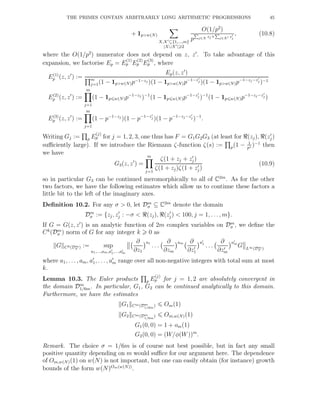
![46 BEN GREEN AND TERENCE TAO
Proof. First consider j = 1. From (10.8) and Taylor expansion we have the crude bound
E
(1)
p (z, z′
) = 1 + Om(p−2+4/6m
) in Dm
1/6m, which gives the desired convergence and also
the Cm
(Dm
1/6m) bound on G1; the estmate for G1(0, 0) also follows since the Euler factors
E
(1)
p (z, z′
) are identically 1 when p w(N). The bound for G2 are easy since this is just
a finite Euler product involving at most w(N) terms; the formula for G2(0, 0) follows
from direct calculation since φ(W )
W
= p<w(n)(1 − 1
p
).
To estimate (10.5), we now invoke the following contour integration lemma.
Lemma 10.4. [17] Let R be a positive real number. Let G = G(z, z′
) be an analytic
function of 2m complex variables on the domain Dm
σ for some σ > 0, and suppose that
G Cm(Dm
σ ) = exp(Om,σ(log1/3
R)). (10.10)
Then
1
(2πi)2m
Γ1
. . .
Γ1
G(z, z′
)
m
j=1
ζ(1 + zj + z′
j)
ζ(1 + zj)ζ(1 + z′
j)
Rzj+z′
j
z2
j z′2
j
dzjdz′
j
= G(0, . . ., 0) logm
R +
m
j=1
Om,σ( G Cj(Dm
σ ) logm−j
R) + Om,σ(e−δ
√
log R
)
for some δ = δ(m) > 0.
Proof. While this lemma is essentially in [17], we shall give a complete proof in the
Appendix for sake of completeness.
We apply this lemma with G := G1G2 and σ := 1/6m. From Lemma 10.3 and the
Leibnitz rule we have the bounds
G Cj(Dm
1/6m
) Oj,m,w(N)(1) for all 0 j m,
and in particular we obtain (10.10) by choosing w(N) to grow sufficiently slowly in N.
Also we have G(0, 0) = (1+om(1))( W
φ(W )
)m
from that lemma. We conclude (again taking
w(N) sufficiently slowly growing in N) that the quantity in (10.5) is (1+om(1))(W log R
φ(W )
)m
,
as desired. This concludes the proof of Proposition 9.5.
Higher order correlations for ΛR. We now prove Proposition 9.6, using arguments very
similar to those used to prove Proposition 9.5. The main differences here are that the
number of variables t is just equal to 1, but on the other hand all the linear forms are
equal to each other, ψi(x1) = x1. In particular, these linear forms are now rational
multiples of each other and so Lemma 10.1 no longer applies. However, the arguments
before that Lemma are still valid; thus we can still write the left-hand side of (9.1) as
an expression of the form (10.5) plus an acceptable error, where F is again defined by
(10.6) and Ep is defined by (10.7); the difference now is that ωX(p) is the quantity
ωX(p) := E
i∈X
1W (x+hi)+1≡0(mod p) x ∈ Zp .
Again we have ω∅(p) = 1 for all p. The analogue of Lemma 10.1 is as follows.](https://image.slidesharecdn.com/theprimescontainarbitrarilylongarithmeticprogressions-180218024935/85/Teorema-de-Green-Tao-46-320.jpg)
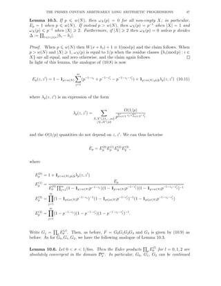
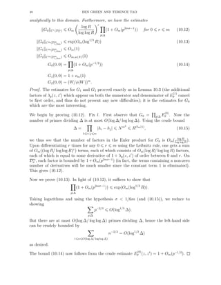
![THE PRIMES CONTAIN ARBITRARILY LONG ARITHMETIC PROGRESSIONS 49
We now apply Lemma 10.4 with σ := 1/6m and G := G0G1G2. Again by the Leibnitz
rule we have the bound (10.10), and furthermore
G Cr(Dm
σ ) Om(1)Om,w(N)(1)
log R
log log R
r
p|∆
1 + Om(p−1/2
) .
for all 0 r m. From Lemma 10.6 and Lemma 10.4 we can then estimate (10.5) as
(1 + om(1))
W
φ(W)
m
logm
R
p|∆
1 + Om(p−1/2
)
+ Om,w(N)
logm
R
log log R
p|∆
1 + Om(p−1/2
) + Om(e−δ
√
log R
).
The claim (9.1) then follows by choosing w(N) (and hence W) sufficiently slowly growing
in N (and hence in R). Proposition 9.6 follows.
Remark. It should be clear that the above argument not only gives an upper bound
for the left-hand side of (9.1), but in fact gives an asymptotic, by working out G0(0, 0)
more carefully; this is worked out in detail (in the W = 1 case) in [17].
11. Further remarks
In this section we discuss some extensions and refinements of our main result. First
of all, notice that our proof actually shows that that there is some constant γ(k) such
that the number of k-term progressions of primes, all less than N, is at least (γ(k) +
o(1))N2
/ logk
N. This is because the error term in (3.9) does not actually need to be
o(1), but merely less than 1
2
c(k, δ) + o(1) (for instance). Working backwards through
the proof, this eventually reveals that the quantity w(N) does not actually need to
be growing in N, but can instead be a fixed number depending only on k (although
this number will be very large because our final bounds o(1) decayed to zero extremely
slowly). Thus W can be made independent of N, and so the loss incurred by the W-
trick when passing from primes to primes equal to 1 mod W is bounded uniformly in
N. Nevertheless the bound we obtain on γ(k) is extremely poor, in part because of the
growth of constants in the best known bounds c(k, δ) on Szemer´edi’s theorem in [19],
but also because we have not attempted to optimise the decay rate of the o(1) factors
and hence will need to take w(N) to be extremely large. In the other direction, standard
sieve theory arguments show that the number of k-term progressions of primes all less
than N are at most Ok(N2
/ logk
N), and so the lower bounds are only off by a constant
depending on k.
As we remarked earlier, our method also extends to prove Theorem 1.2, namely that any
subset of the primes with positive relative upper density contains a k-term arithmetic
progression. The only significant change23
to the proof is that one must use the pigeon-
hole principle to replace the residue class n ≡ 1(mod W) by a more general residue class
n ≡ b(mod W) for some b coprime to W, since the set A in Theorem 1.2 does not need
23Also, since we are only assuming positivity of the upper density and not the lower density, we
only have good density control for an infinite sequence N1, N2, . . . → ∞ of integers, which may not be
prime. However one can easily use Bertrands postulate (for instance) to make the Nj prime, giving up
a factor of O(1) at most.](https://image.slidesharecdn.com/theprimescontainarbitrarilylongarithmeticprogressions-180218024935/85/Teorema-de-Green-Tao-49-320.jpg)
![50 BEN GREEN AND TERENCE TAO
to obey a Dirichlet-type theorem in these residue classes. However it is easy to verify
that this does not significantly affect the rest of the argument, and we leave the details
to the reader.
Applying Theorem 1.2 to the set of primes p ≡ 1(mod 4), we obtain the previously
unknown fact that there are arbitrarily long progressions consisting of numbers which
are the sum of two squares. For this problem, more satisfactory results were known for
small k than was the case for the primes. Let S be the set of sums of two squares. It is a
simple matter to show that there are infinitely many 4-term arithmetic progressions in S.
Indeed, Heath-Brown [26] observed that the numbers (n−1)2
+(n−8)2
, (n−7)2
+(n+4)2
,
(n+7)2
+(n−4)2
and (n+1)2
+(n+8)2
always form such a progression; in fact, he was
able to prove much more, in particular finding an asymptotic for the number of 4-term
progressions in S, all of whose members are at most N (weighted by r(n), the number
of representations of n as the sum of two squares).
It is reasonably clear that our method will produce long arithmetic progressions for
many sets of primes for which one can give a lower bound which agrees with some
upper bound coming from a sieve, up to a multiplicative constant. Invoking Chen’s
famous theorem[7] to the effect that there are ≫ N/ log2
N primes p N for which
p + 2 is a prime or a product of two primes, it ought to be a simple matter to adapt
our arguments to show that there are arbitrarily long arithmetic progressions p1, . . . , pk
of primes, such that each pi + 2 is either prime or the product of two primes; indeed
there should be N/ log2k
N such progressions with entries less than N. Whilst we do
not plan24
to write a detailed proof of this fact, we will in [23] give a proof of the case
k = 3 using harmonic analysis.
The methods in this paper suggest a more general “transference principle”, in that if
a type of pattern (such as an arithmetic progression) is forced to arise infinitely often
within sets of positive density, then it should also be forced to arise infinitely often
inside the prime numbers, or more generally inside any subset of a pseudorandom set
(such as the “almost primes”) of positive relative density. Thus, for instance, one is
led to conjecture a Bergelson-Leibman type result (cf. [4]) for primes. That is, one
could hope to show that if Fi : N → N are polynomials with F(0) = 0, then there are
infinitely many configurations (a + F1(d), . . ., a + Fk(d)) in which all k elements are
prime. This however seems to require some modification25
to our current argument,
in large part because of the need to truncate the step parameter d to be at most a
small power of N. In a similar spirit, the work of Furstenberg and Katznelson [11] on
multidimensional analogues of Szemer´edi’s theorem, combined with this transference
principle, now suggests that one should be able to show26
that the Gaussian primes in
Z[i] contain infinitely many constellations of any prescribed shape, and similarly for
24Very briefly, the idea is to replace the function ΛR(Wn + 1) in the definition of the pseudorandom
measure ν with a variant such as ΛR(Wn+b)ΛR(Wn+b+2) for some 1 b < W for which b, b+2 are
both coprime to W; one can use Chen’s theorem and the pigeonhole principle to locate a b for which
this majorant will capture a large number of Chen primes. We leave the details to the reader.
25Note added in press: such a result has been obtained by the second author and T. Ziegler, to
appear in Acta Math.
26Note added in press: such a result has been obtained by the second author, J. d’Analyse
Math´ematique 99 (2006), 109–176.](https://image.slidesharecdn.com/theprimescontainarbitrarilylongarithmeticprogressions-180218024935/85/Teorema-de-Green-Tao-50-320.jpg)
![THE PRIMES CONTAIN ARBITRARILY LONG ARITHMETIC PROGRESSIONS 51
other number fields. Furthermore, the later work of Furstenberg and Katznelson [12]
on density Hales-Jewett theorems suggests that one could also show that for any finite
field F, the monic irreducible polynomials in F[t] contain affine subspaces over F of
arbitrarily high dimension. Again, these results would require non-trivial modifications
to our argument for a number of reasons, not least of which is the fact that the char-
acteristic factors for these more advanced generalizations of Szemer´edi’s theorem are
much less well understood.
Appendix A. Proof of Lemma 10.4
In this appendix we prove Lemma 10.4. This Lemma was essentially proven in [17],
but for the sake of self-containedness we provide a complete proof here (following very
closely the approach in [17]).
Throughout this section, R 2, m 1, and σ > 0 will be fixed. We shall use
δ > 0 to denote various small constants, which may vary from line to line (the previous
interpretation of δ as the average value of a function f will now be irrelevant). We begin
by recalling the classical zero-free region for the Riemann ζ function.
Lemma A.1 (Zero-free region). Define the classical zero free region Z to be the closed
region
Z := {s ∈ C : 10 ℜs 1 −
β
log(|ℑs| + 2)
}
for some small 0 < β < 1. Then if β is sufficiently small, ζ is non-zero and meromorphic
in Z with a simple pole at 1 and no other singularities. Furthermore we have the bounds
ζ(s) −
1
s − 1
= O(log(|ℑs| + 2));
1
ζ(s)
= O(log(|ℑs| + 2))
for all s ∈ Z.
Proof. See Titchmarsh [41, Chapter 3].
Fix β in the above lemma; we may take β to be small enough that Z is contained
in the region where 1 − σ < ℜ(s) < 101. We will allow all our constants in the O()
notation to depend on β and σ, and omit explicit mention of these dependencies from
our subscripts.
In addition to the contour Γ1 defined in (10.4), we will need the two further contours
Γ0 and Γ2, defined by
Γ0(t) := −
β
log(|t| + 2)
+ it, −∞ < t < ∞
Γ2(t) := 1 + it, −∞ < t < ∞.
(A.1)
Thus Γ0 is the left boundary of Z − 1 (which therefore lies to the left of the origin),
while Γ1 and Γ2 are vertical lines to the right of the origin. The usefulness of Γ2 for
us lies in the simple observation that ζ(1 + z + z′
) has no poles when z ∈ Z − 1 and
z′
∈ Γ2, but we will not otherwise attempt to estimate any integrals on Γ2.
We observe the following elementary integral estimates.](https://image.slidesharecdn.com/theprimescontainarbitrarilylongarithmeticprogressions-180218024935/85/Teorema-de-Green-Tao-51-320.jpg)
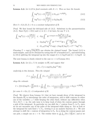
![THE PRIMES CONTAIN ARBITRARILY LONG ARITHMETIC PROGRESSIONS 53
have I = I1 + I2, where
I1 :=
1
2πi Γ2
f(0, z′
)
Rz′
z′2
dz′
I2 :=
1
(2πi)2
Γ2 Γ0
f(z, z′
)
ζ(1 + z + z′
)Rz+z′
ζ(1 + z)ζ(1 + z′)z2z′2
dzdz′
.
To evaluate I1, we shift the z′
contour of integration to Γ0. Again there is just one pole,
a double one at z′
= 0. The residue there is f(0, 0) log R + ∂f
∂z′ (0, 0), and so
I1 = f(0, 0) log R +
∂f
∂z′
(0, 0) +
1
2πi Γ0
f(0, z′
)
Rz′
z′2
dz′
= f(0, 0) log R +
∂f
∂z′
(0, 0) + Om(e−δ
√
log R
),
for some δ > 0, the latter step being a consequence of our bound on f and (A.2) (in
the case B = 0).
To estimate I2, we first swap the order of integration and, for each fixed z, view the
integrand as an analytic function of z′
. We move the z′
contour from Γ2 to Γ0, this
again being allowed since we have sufficient decay in vertical strips as |ℑz′
| → ∞. In so
doing we pass exactly two simple poles, at z′
= −z and z′
= 0. The residue at the first
is exactly
1
2πi Γ0
f(z, −z)
dz
ζ(1 + z)ζ(1 − z)z4
,
which is one of the terms appearing in our formula for I.
The residue at z′
= 0 is
Γ0
f(z, 0)
Rz
z2
dz,
which is O(e−δ
√
log R
) for some δ > 0 by (A.2). The value of I2 is the sum of these two
quantities and the integral over the new contour Γ0, which is
Γ0 Γ0
f(z, z′
)
ζ(1 + z + z′
)Rz+z′
ζ(1 + z)ζ(1 + z′)z2z′2
dzdz′
. (A.4)
In this integrand we have |f| = exp(Om(log1/3
R)) and, by Lemma A.1, 1/|ζ(1 + z)| ≪
log(|ℑz| + 2) and 1/|ζ(1 + z′
)| ≪ log(|ℑz′
| + 2). Assume that β < 1/10, as we obviously
may. We claim that
|ζ(1 + z + z′
)| ≪ (1 + |z| + |z′
|)1/4
≪ (1 + |z|)1/4
(1 + |z′
|)1/4
(A.5)
for all z, z′
∈ Γ0. Once this is proven it follows from (A.2), applied with A = 7/4 and
A = 2, that the integral (A.4) is bounded by Om(e−δ
√
log R
) for some δ > 0. Now if
1/2 σ 1 and |t| 1/100 we have the convexity bound |ζ(σ + it)| ≪ǫ |t|1−σ+ǫ
(cf.
[41, Chapter V]), and so (A.5) is indeed true provided that |ℑ(z+z′
)| 1/100. However
since z, z′
∈ Γ0 one may see that if |ℑ(z)|, |ℑ(z′
)| t then |z + z′
| ≫ 1/ log(t + 2). It
follows from Lemma A.1 that (A.5) holds when |ℑ(z + z′
)| 1/100 as well.
Thus we now have estimates for I1 and I2 up to errors of Om(e−δ
√
log R
). Putting all of
this together completes the proof of the lemma.](https://image.slidesharecdn.com/theprimescontainarbitrarilylongarithmeticprogressions-180218024935/85/Teorema-de-Green-Tao-53-320.jpg)
![THE PRIMES CONTAIN ARBITRARILY LONG ARITHMETIC PROGRESSIONS 55
for 0 j m. Using the inductive hypothesis, we therefore obtain I(G, m + 1) =
G(0, . . ., 0)(log R)m+1
+
m
j=1
Om( G(·, 0, ·, 0) Cj(Dm
σ )(log R)m+1−j
)
+H(0, . . ., 0)(log R)m
+
m
j=1
Om( H Cj(Dm
σ )(log R)m−j
) + O(e−δ
√
log R
)
= G(0, . . ., 0)(log R)m+1
+
m
j=1
Om( G Cj(Dm+1
σ )(log R)m+1−j
)
+H(0, . . ., 0)(log R)m
+
m
j=1
Om( G Cj+1(Dm+1
σ )(log R)m−j
) + O(e−δ
√
log R
)
= G(0, . . ., 0)(log R)m+1
+
m+1
j=1
Om( G Cj(Dm+1
σ )(log R)m+1−j
) + O(e−δ
√
log R
),
which is what we wanted to prove.
References
[1] I. Assani, Pointwise convergence of ergodic averages along cubes, preprint.
[2] A. Balog, Linear equations in primes, Mathematika 39 (1992) 367–378.
[3] , Six primes and an almost prime in four linear equations, Can. J. Math. 50 (1998), 465–
486.
[4] V. Bergelson and A. Leibman, Polynomial extensions of van der Waerden’s and Szemer´edi’s the-
orems, J. Amer. Math. Soc. 9 (1996), 725–753.
[5] J. Bourgain, A Szemer´edi-type theorem for sets of positive density in Rk
, Israel J. Math 54 (1986),
no. 3, 307–316.
[6] , On triples in arithmetic progression, GAFA 9 (1999), 968–984.
[7] J.-R. Chen, On the representation of a large even integer as the sum of a prime and a product of
at most two primes, Sci. Sinica 16 (1973), 157–176.
[8] S. Chowla, There exists an infinity of 3—combinations of primes in A. P., Proc. Lahore Philos.
Soc. 6, (1944). no. 2, 15–16.
[9] P. Erd˝os, P. Tur´an, On some sequences of integers, J. London Math. Soc. 11 (1936), 261–264.
[10] H. Furstenberg, Ergodic behavior of diagonal measures and a theorem of Szemer´edi on arithmetic
progressions, J. Analyse Math. 31 (1977), 204–256.
[11] H. Furstenberg, Y. Katznelson, An ergodic Szemer´edi theorem for commuting transformations. J.
Analyse Math. 34 (1978), 275–291.
[12] H. Furstenberg, Y. Katznelson, A density version of the Hales-Jewett theorem, J. d’Analyse Math.
57 (1991), 64–119.
[13] H. Furstenberg, Y. Katznelson and D. Ornstein, The ergodic-theoretical proof of Szemer´edi’s the-
orem, Bull. Amer. Math. Soc. 7 (1982), 527–552.
[14] H. Furstenberg, B. Weiss, A mean ergodic theorem for 1/N
N
n=1 f(T n
x)g(T n2
x), Convergence in
ergodic theory and probability (Columbus OH 1993), 193–227, Ohio State Univ. Math. Res. Inst.
Publ., 5. de Gruyter, Berlin, 1996.
[15] D. Goldston and C.Y. Yıldırım Higher correlations of divisor sums related to primes, I: Triple
correlations, Integers 3 (2003) A5, 66pp.
[16] , Higher correlations of divisor sums related to primes, III: k-correlations, preprint (avail-
able at AIM preprints)
[17] , Small gaps between primes, I, preprint available at
http://www.arxiv.org/abs/math/0504336.](https://image.slidesharecdn.com/theprimescontainarbitrarilylongarithmeticprogressions-180218024935/85/Teorema-de-Green-Tao-55-320.jpg)
![56 BEN GREEN AND TERENCE TAO
[18] T. Gowers, A new proof of Szemer´edi’s theorem for arithmetic progressions of length four, GAFA
8 (1998), 529–551.
[19] , A new proof of Szemer´edi’s theorem, GAFA 11 (2001), 465-588.
[20] , Hypergraph regularity and the multidimensional Szemer´edi theorem, preprint.
[21] B.J. Green, Roth’s theorem in the primes, Ann. Math. 161 (2005), no. 3, 1609–1636.
[22] , A Szemer´edi-type regularity lemma in abelian groups, GAFA 15 (2005), no. 2, 340–376.
[23] B.J. Green and T. Tao, Restriction theory of Selberg’s sieve, with applications, J. Th´eorie des
Nombres de Bordeaux 18 (2006), 147–182.
[24] G.H. Hardy and J.E. Littlewood Some problems of “partitio numerorum”; III: On the expression
of a number as a sum of primes, Acta Math. 44 (1923), 1–70
[25] D.R. Heath-Brown, Three primes and an almost prime in arithmetic progression, J. London Math.
Soc. (2) 23 (1981), 396–414.
[26] , Linear relations amongst sums of two squares, Number theory and algebraic geometry —
to Peter Swinnerton-Dyer on his 75th birthday, CUP (2003).
[27] B. Host and B. Kra, Convergence of Conze-Lesigne averages, Ergodic Theory and Dynamical
Systems 21 (2001), no. 2, 493–509.
[28] , Non-conventional ergodic averages and nilmanifolds, Ann. Math. 161 (2005), no. 1, 397–
488.
[29] , Convergence of polynomial ergodic averages, Israel. Jour. Math. 149 (2005), 1–19.
[30] Y. Kohayakawa, T. Luczsak, V. R¨odl, Arithmetic progressions of length three in subsets of a
random set, Acta Arith. 75 (1996), no. 2, 133–163.
[31] I. Laba and M. Lacey, On sets of integers not containing long arithmetic progressions, unpublished.
Available at http://www.arxiv.org/pdf/math.CO/0108155.
[32] A. Moran, P. Pritchard and A. Thyssen, Twenty-two primes in arithmetic progression, Math.
Comp. 64 (1995), no. 211, 1337–1339.
[33] O. Ramar´e, On Snirel’man’s constant, Ann. Scu. Norm. Pisa 21 (1995), 645–706.
[34] O. Ramar´e and I.Z. Ruzsa, Additive properties of dense subsets of sifted sequences, J. Th. Nombres
de Bordeaux 13 (2001) 559–581.
[35] R. Rankin, Sets of integers containing not more than a given number of terms in arithmetical
progression. Proc. Roy. Soc. Edinburgh Sect. A, 65 1960/1961 332–344 (1960/61).
[36] K.F. Roth, On certain sets of integers, J. London Math. Soc. 28 (1953), 245-252.
[37] E. Szemer´edi, On sets of integers containing no four elements in arithmetic progression, Acta
Math. Acad. Sci. Hungar. 20 (1969), 89–104.
[38] , On sets of integers containing no k elements in arithmetic progression, Acta Arith. 27
(1975), 299–345.
[39] , Regular partitions of graphs, in “Proc. Colloque Inter. CNRS” (J.-C. Bermond, J.-C.
Fournier, M. Las Vergnas, D. Sotteau, eds.) (1978), 399–401.
[40] T. Tao, A quantitative ergodic theory proof of Szemer´edi’s theorem, to appear in Electronic J.
Combinatorics.
[41] E.C. Titchmarsh, The theory of the Riemann zeta function, Oxford University Press, 2nd ed, 1986.
[42] J.G. van der Corput, ¨Uber Summen von Primzahlen und Primzahlquadraten, Math. Ann. 116
(1939), 1–50.
[43] P. Varnavides, On certain sets of positive density, J. London Math. Soc. 34 (1959) 358–360.
[44] T. Ziegler, Universal characteristic factors and Furstenberg averages, J. Amer. Math. Soc. 20
(2007), no. 1, 53–97.
[45] , A non-conventional ergodic theorem for a nilsystem, A non-conventional ergodic theorem
for a nilsystem. Ergodic Theory Dynam. Systems 25 (2005), no. 4, 1357–1370.
School of Mathematics, University Walk, Bristol, BS8 1TW
E-mail address: b.j.green@bristol.ac.uk
Department of Mathematics, University of California at Los Angeles, Los Angeles
CA 90095
E-mail address: tao@math.ucla.edu](https://image.slidesharecdn.com/theprimescontainarbitrarilylongarithmeticprogressions-180218024935/85/Teorema-de-Green-Tao-56-320.jpg)

This document summarizes a proof that the prime numbers contain arbitrarily long arithmetic progressions. The proof has three main ingredients: 1) Szemerédi's theorem, which states that any subset of integers with positive density contains long arithmetic progressions; 2) a transference principle showing that pseudorandom sets also contain long progressions; 3) a result of Goldston and Yıldırım showing that almost all primes lie in a pseudorandom set. The document outlines how these ingredients can be combined to prove the main theorems that prime numbers contain arbitrarily long progressions and any subset of primes with positive density contains long progressions.