![Experimental realisation of Shor’s quantum factoring algorithm using qubit recycling
Enrique Mart´ın-L´opez,∗
Anthony Laing,∗
Thomas Lawson,∗
Roberto Alvarez, Xiao-Qi Zhou, and Jeremy L. O’Brien†
Centre for Quantum Photonics, H. H. Wills Physics Laboratory & Department of Electrical and Electronic Engineering,
University of Bristol, Merchant Venturers Building, Woodland Road, Bristol, BS8 1UB, UK
Quantum computational algorithms exploit quantum mechanics to solve problems exponentially
faster than the best classical algorithms1–3
. Shor’s quantum algorithm4
for fast number factoring is
a key example and the prime motivator in the international effort to realise a quantum computer5
.
However, due to the substantial resource requirement, to date, there have been only four small-scale
demonstrations6–9
. Here we address this resource demand and demonstrate a scalable version of
Shor’s algorithm in which the n qubit control register is replaced by a single qubit that is recycled
n times: the total number of qubits is one third of that required in the standard protocol10–12
.
Encoding the work register in higher-dimensional states, we implement a two-photon compiled
algorithm to factor N = 21. The algorithmic output is distinguishable from noise, in contrast to
previous demonstrations. These results point to larger-scale implementations of Shor’s algorithm
by harnessing scalable resource reductions applicable to all physical architectures.
Shor’s factoring algorithm consists of a quantum or-
der finding algorithm, preceded and succeeded by various
classical routines. While the classical tasks are known
to be efficient on a classical computer, order finding is
understood to be intractable classically. However, it is
known that this part of the algorithm can be performed
efficiently on a quantum computer. To determine the
prime factors of an odd integer N, one chooses a co-
prime of N, x. The order r relates x to N according to xr
mod N = 1, and can be used to obtain the factors, given
by the greatest common divisor gcd(x
r
2 ± 1, N).
The quantum order finding circuit involves two reg-
isters: a work register and a control register. In the
standard protocol, the work register performs modular
arithmetic with m = log2 N qubits, enough to encode
the number N, and the n qubit control register provides
the algorithmic output, with n bits of precision.
Measuring the control register in the computational
basis will yield a result of k2n
/r where k is an integer
between 0 and r−1, with the value of k occurring proba-
bilistically. Dividing the result by 2n
gives the first n bits
of k/r and r may be found with classical processing, us-
ing the continued fraction algorithm. For large n, and a
perfectly functioning circuit, the output probability dis-
tribution of the control register is a series of well defined
peaks at values of k2n
/r (Fig. 1b). (See Appendix for
details.)
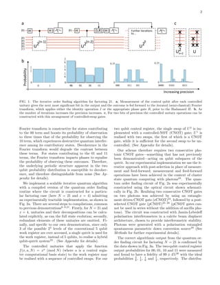
Here we implement an iterative version of the order
finding algorithm10,11
, in which the control register con-
tains only a single qubit which is recycled n times, using
a sequence of measurement and feed-forward operations,
with each step providing an additional bit of precision
(Fig. 1a). Reducing the number of qubits in quantum
simulations and quantum chemistry has been achieved
with recursive phase estimation13–16
, while ground state
projections have been demonstrated by exploiting similar
techniques in NMR17
.
The iterative version of the order finding algorithm,
displayed in Fig. 1a, is closely related to the semi-classical
picture of the quantum Fourier transform18
. Rather than
performing a Fourier transformation across all control
register qubits simultaneously, it is sufficient to measure
the coherence between computational basis states of in-
dividual qubits in the control register (from least signifi-
cant bit to greatest significant bit) deciding on the phase
coherence of the next measurement depending on the pre-
vious result. In fact, the control register need not contain
more than one qubit at any one time. This register be-
gins in a product state and all unitaries controlled from
the (i)th control qubit are performed before those con-
trolled from the (i+1)th control qubit. This means that
all operations on the (i)th qubit can be performed before
the (i+1)th qubit is initialised and a single control qubit
can be re-used, or recycled, with the state of the work
register iteratively updated at each stage.
To guarantee a good level of precision in k/r, a full
scale implementation of Shor’s algorithm requires n to
be log(N2
) n log(2N2
). So for full scale imple-
mentations, qubit recycling reduces the total number of
qubits required from 3 log2 N to log2 N + 1; the only
penalty is a polynomial increase in computation time,
while the exponential speedup is retained—i.e. it is scal-
able. In general, saving in qubits can be more than 2/3
if more control qubits are required, or less than 2/3 in
smaller proof of principle demonstrations such as this.
As the number of control qubits, or iterations, n is
reduced, in general, the precision is reduced and the k
peaks in the probability distribution become smeared, as
shown in Fig. 1b. However, in the special case where
the order is a power of two and r = 2p
, the peaks cor-
respond exactly to the logical states of p qubits19
such
that the output is equivalent to that of an incoherent
mixture of p qubits (any additional control qubits re-
main unentangled throughout the algorithm and simply
encode the trailing zeros in the uniform distribution).
Factoring N = 15 gives either order 2 or order 4 for each
of its co-primes6–9
; independent verification of entangle-
ment is therefore required7,8
. For this reason we focus on
N = 21 with the co-prime x = 4 to give order20
r = 3.
To two bits of precision the expected outcomes 00,
01, 10 and 11 occur with probabilities 3
8 , 1
4 , 1
8 and
1
4 , respectively (Fig 1b). Quantum interference in the
arXiv:1111.4147v2[quant-ph]24Oct2012](https://image.slidesharecdn.com/experimentalrealisationofshorsquantumfactoringalgorithmusingqubitrecycling-180504235701/85/Experimental-realisation-of-Shor-s-quantum-factoring-algorithm-using-qubit-recycling-1-320.jpg)
![Experimental realisation of Shor’s quantum factoring algorithm using qubit recycling
Enrique Mart´ın-L´opez,∗
Anthony Laing,∗
Thomas Lawson,∗
Roberto Alvarez, Xiao-Qi Zhou, and Jeremy L. O’Brien†
Centre for Quantum Photonics, H. H. Wills Physics Laboratory & Department of Electrical and Electronic Engineering,
University of Bristol, Merchant Venturers Building, Woodland Road, Bristol, BS8 1UB, UK
Quantum computational algorithms exploit quantum mechanics to solve problems exponentially
faster than the best classical algorithms1–3
. Shor’s quantum algorithm4
for fast number factoring is
a key example and the prime motivator in the international effort to realise a quantum computer5
.
However, due to the substantial resource requirement, to date, there have been only four small-scale
demonstrations6–9
. Here we address this resource demand and demonstrate a scalable version of
Shor’s algorithm in which the n qubit control register is replaced by a single qubit that is recycled
n times: the total number of qubits is one third of that required in the standard protocol10–12
.
Encoding the work register in higher-dimensional states, we implement a two-photon compiled
algorithm to factor N = 21. The algorithmic output is distinguishable from noise, in contrast to
previous demonstrations. These results point to larger-scale implementations of Shor’s algorithm
by harnessing scalable resource reductions applicable to all physical architectures.
Shor’s factoring algorithm consists of a quantum or-
der finding algorithm, preceded and succeeded by various
classical routines. While the classical tasks are known
to be efficient on a classical computer, order finding is
understood to be intractable classically. However, it is
known that this part of the algorithm can be performed
efficiently on a quantum computer. To determine the
prime factors of an odd integer N, one chooses a co-
prime of N, x. The order r relates x to N according to xr
mod N = 1, and can be used to obtain the factors, given
by the greatest common divisor gcd(x
r
2 ± 1, N).
The quantum order finding circuit involves two reg-
isters: a work register and a control register. In the
standard protocol, the work register performs modular
arithmetic with m = log2 N qubits, enough to encode
the number N, and the n qubit control register provides
the algorithmic output, with n bits of precision.
Measuring the control register in the computational
basis will yield a result of k2n
/r where k is an integer
between 0 and r−1, with the value of k occurring proba-
bilistically. Dividing the result by 2n
gives the first n bits
of k/r and r may be found with classical processing, us-
ing the continued fraction algorithm. For large n, and a
perfectly functioning circuit, the output probability dis-
tribution of the control register is a series of well defined
peaks at values of k2n
/r (Fig. 1b). (See Appendix for
details.)
Here we implement an iterative version of the order
finding algorithm10,11
, in which the control register con-
tains only a single qubit which is recycled n times, using
a sequence of measurement and feed-forward operations,
with each step providing an additional bit of precision
(Fig. 1a). Reducing the number of qubits in quantum
simulations and quantum chemistry has been achieved
with recursive phase estimation13–16
, while ground state
projections have been demonstrated by exploiting similar
techniques in NMR17
.
The iterative version of the order finding algorithm,
displayed in Fig. 1a, is closely related to the semi-classical
picture of the quantum Fourier transform18
. Rather than
performing a Fourier transformation across all control
register qubits simultaneously, it is sufficient to measure
the coherence between computational basis states of in-
dividual qubits in the control register (from least signifi-
cant bit to greatest significant bit) deciding on the phase
coherence of the next measurement depending on the pre-
vious result. In fact, the control register need not contain
more than one qubit at any one time. This register be-
gins in a product state and all unitaries controlled from
the (i)th control qubit are performed before those con-
trolled from the (i+1)th control qubit. This means that
all operations on the (i)th qubit can be performed before
the (i+1)th qubit is initialised and a single control qubit
can be re-used, or recycled, with the state of the work
register iteratively updated at each stage.
To guarantee a good level of precision in k/r, a full
scale implementation of Shor’s algorithm requires n to
be log(N2
) n log(2N2
). So for full scale imple-
mentations, qubit recycling reduces the total number of
qubits required from 3 log2 N to log2 N + 1; the only
penalty is a polynomial increase in computation time,
while the exponential speedup is retained—i.e. it is scal-
able. In general, saving in qubits can be more than 2/3
if more control qubits are required, or less than 2/3 in
smaller proof of principle demonstrations such as this.
As the number of control qubits, or iterations, n is
reduced, in general, the precision is reduced and the k
peaks in the probability distribution become smeared, as
shown in Fig. 1b. However, in the special case where
the order is a power of two and r = 2p
, the peaks cor-
respond exactly to the logical states of p qubits19
such
that the output is equivalent to that of an incoherent
mixture of p qubits (any additional control qubits re-
main unentangled throughout the algorithm and simply
encode the trailing zeros in the uniform distribution).
Factoring N = 15 gives either order 2 or order 4 for each
of its co-primes6–9
; independent verification of entangle-
ment is therefore required7,8
. For this reason we focus on
N = 21 with the co-prime x = 4 to give order20
r = 3.
To two bits of precision the expected outcomes 00,
01, 10 and 11 occur with probabilities 3
8 , 1
4 , 1
8 and
1
4 , respectively (Fig 1b). Quantum interference in the
arXiv:1111.4147v2[quant-ph]24Oct2012](https://image.slidesharecdn.com/experimentalrealisationofshorsquantumfactoringalgorithmusingqubitrecycling-180504235701/75/Experimental-realisation-of-Shor-s-quantum-factoring-algorithm-using-qubit-recycling-1-2048.jpg)
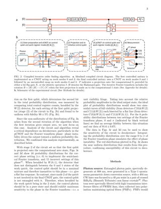

The document presents a scalable experimental realization of Shor's quantum factoring algorithm, implementing a qubit recycling technique that reduces the required number of qubits by two-thirds while preserving computational efficiency. By utilizing a two-photon compiled algorithm, the research successfully factors the number 21, demonstrating distinguishable results from noise and advocating for larger-scale implementations of Shor's algorithm. The iterative approach, combined with a single control qubit recycled multiple times, allows for increased precision in output while maintaining the algorithm's exponential speedup.


![ANIMAL_CELL_,_TISSUE_AND_ORGAN_CULTURE[1].pptx](https://cdn.slidesharecdn.com/ss_thumbnails/animalcelltissueandorganculture1-260204172026-4462b440-thumbnail.jpg?width=640&height=640&fit=bounds)


